Clarification
Diffusion model involves quite a bit math. So we take a particular format of slides that
- Detailed derivations are bracketed by two labels: "EXTRA -->" and "<-- EXTRA".
- You may skip these in the first round of learning
- The rest slides are self-contained and capture the main ideas and key results
If you press
esc, you would see a 2D grid of slides, from which it might be easier to see the EXTRA labels.
A good portion of formulation is based on DDPM.
However, for a general treatment, we used notations that are closer to EDM.
Basic Idea
 (Figure from Yang2024)
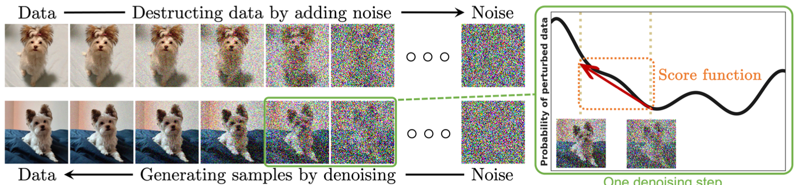
- Top row: A forward process, that sequentially and gradually convert data to pure noise.
- Imagine we put a drop of ink in a cup of water, over time the ink diffuse evenly into the entire cup
- Bottom row: A backward process, that "magically" reverts the above process.
- As if we get a cup of ink-water, and revert it to a cup of pure water and a drop of ink.
- Right figure: The "magic", called score function, which we will define later.
- This is the working horse of diffusion model.
Generative Models
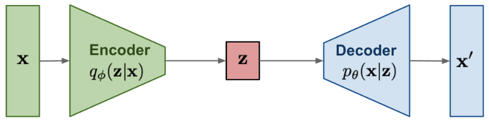
DM is a type of generative models. Earlier we encountered another generative model, Variational Autoencoder (VAE)
 (lilianweng.github.io/posts/2021-07-11-diffusion-models/)
- At the inference stage, we sample from a unit Gaussian distribution ($z$), and decode it to a data point $x$ that "looks like" our training data.
- Technically, we map Gaussian distribution to the data distribution via the decoder.
- Conversely, encoder needs to do the reverse.
- The encoder and decoder are highly nonlinear.
- Hence hard to train.
Schematic for DMs
 (lilianweng.github.io/posts/2021-07-11-diffusion-models/)
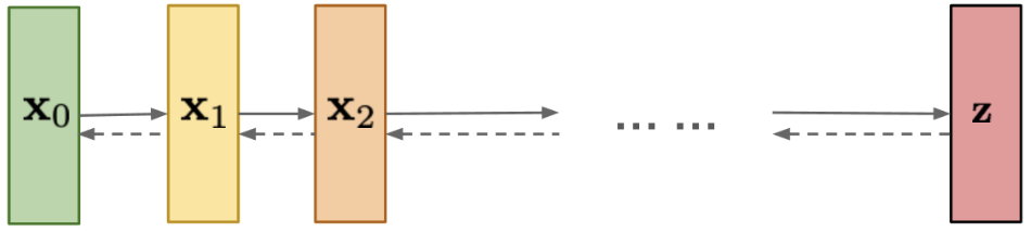
- The forward process functions as an encoder
- The one-step nonlinear mapping of encoder is broken into many-step "linear" mapping
- Later we will see it even has an analytical solution!
- The backward process functions as a decoder
- Again, one-step nonlinear mapping $\Rightarrow$ many-step "linear" mapping
- We just learn one of those "linear" steps
- This should be much easier!
A comprehensive list of applications from [Yang2024]
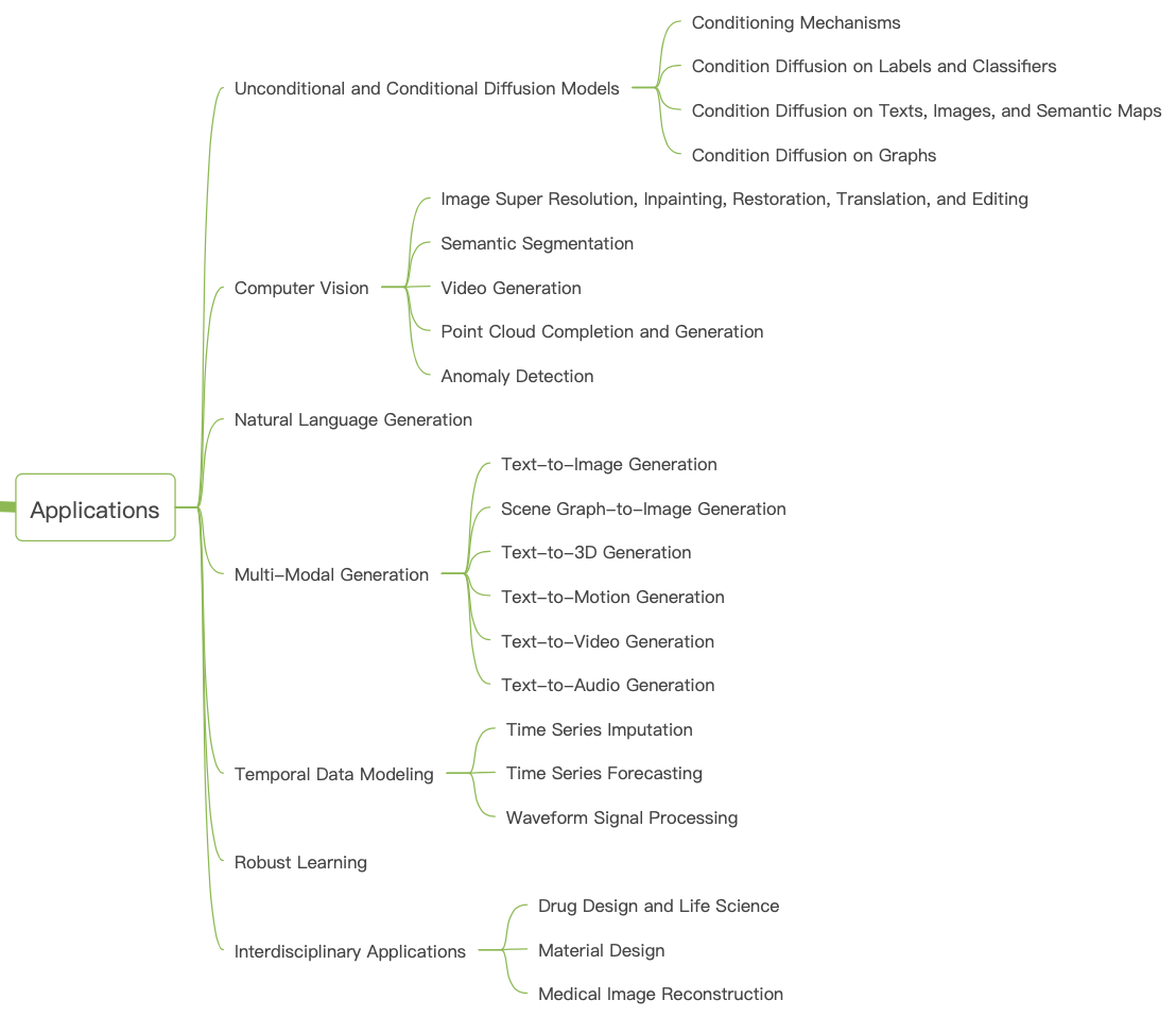
One of the most popular applications is perhaps text-to-image/video generation, e.g., DALL-E, Stable Diffusion, DreamDiffusion.
Formulations
DMs are actually not a new idea, and trace back to, e.g., ICML2015.
Nowadays there are three predominant formulations
- Score-based Generative Model (SGM) - some of the earlier formulations.
- Denoising Diffusion Probabilistic Model (DDPM) - initiated in 2020 and quickly became widely adopted.
- Stochastic differential equation (SDE) - Builds upon and generalizes the previous two formulations.
We will focus on DDPM and SDE, which are discrete and continuous versions of DMs, respectively.
Specifically, we will consider 4 levels of formulations, of increasing depth
- Level 1: Layman version of DDPM
- Level 2: Bayesian version of DDPM
- We will take a break with examples
- Level 3: Generalization to SDE
- Level 4: Connecting to ODE
- After this we will provide more examples
Formulation: Depth Level 1 (of 4)
We will follow the setup in DDPM.
But we will avoid as much probability theory as possible at this level.
The core idea is simple: make the encoder and decoder more gradual.
Encoding: $$ x=x_0\rightarrow x_1\rightarrow x_2\rightarrow \cdots \rightarrow x_{N-1}\rightarrow x_N = z $$
Decoding: $$ z=x_N\rightarrow x_{N-1}\rightarrow x_{N-2}\rightarrow \cdots \rightarrow x_1\rightarrow x_0 = x $$
Let's write down the math for each arrow.
Encoding
Consider a very simple transformation, $$ x_k = A_k x_{k-1} + B_k \epsilon_k,\quad \epsilon_k\sim N(0,I) $$ where
- $\epsilon_k$ is unit Gaussian noise.
- $A_k, B_k$ are scalars and chosen by user
- For later convenience, we require $$ A_k^2+B_k^2=1 $$
EXTRA -->
Then over $k$ steps $$ \begin{align*} x_k &= A_k x_{k-1} + B_k \epsilon_k \\ &= A_k (A_{k-1} x_{k-2} + B_{k-1} \epsilon_{k-1}) + B_k \epsilon_k \\ &= \underbrace{(A_kA_{k-1}\cdots A_1)}_{\equiv\alpha_k}x_0 + \underbrace{ (A_kA_{k-1}\cdots A_2)B_1\epsilon_1 + \cdots + A_kB_{k-1}\epsilon_{k-1} + B_k\epsilon_k }_{\equiv E_k} \end{align*} $$
Since all $e$'s are i.i.d. unit Gaussian, for $E_k$
- The mean is zero
- The variance is $\beta_k^2\equiv 1-\alpha_k^2$, because $$ \begin{align*} &\quad (A_kA_{k-1}\cdots A_2\color{blue}{A_1)^2} + (A_kA_{k-1}\cdots A_2)^2\color{blue}{B_1^2} + (A_kA_{k-1}\cdots A_3)^2B_2^2 + \cdots + A_k^2B_{k-1}^2 + B_k^2 \\ &= (A_kA_{k-1}\cdots\color{green}{A_2)^2} + (A_kA_{k-1}\cdots A_3)^2\color{green}{B_2^2} + \cdots + A_k^2B_{k-1}^2 + B_k^2 \\ &= \cdots \\ &= 1 \end{align*} $$ if we recursively use the relation $A_k^2+B_k^2=1$.
Then we can define $$ E_k = \beta_k\varepsilon_k,\quad \varepsilon_k\sim N(0,I) $$
<-- EXTRA
We can expand out the recursive relation and find $$ x_k = \alpha_k x_0 + \beta_k\varepsilon_k,\quad \varepsilon_k\sim N(0,I) $$
If one design $A_k$ so that $$ \alpha_N \approx 0 $$ then $$ x_N\sim N(0,I) $$
This is exactly what we want: data is destructed into Gaussian noise.
And the best part is
- We do not actually need to implement the encoding process
- The encoding is already "solved" analytically
Decoding
Once encoding is done,
- A sequence of "particular" samples ${\epsilon}_1,\cdots,{\epsilon}_N$ bring $x_0$ to $x_N$
- i.e., $x_{k-1},{\epsilon}_k \Rightarrow x_k$
Then for decoding,
- If we could "guess" the particular ${\epsilon}_k$ for $x_k$, then we can find $x_{k-1}$
- i.e., $x_k,{\epsilon}_k \Rightarrow x_{k-1}$
The guess is done by a neural network with parameter $\theta$, denoted $$ {\epsilon}_k = \epsilon_\theta(x_k) $$ so that, $$ \begin{align*} x_{k-1} &= \frac{1}{A_k}(x_k - B_k\epsilon_k) \\ &= \frac{1}{A_k}(x_k - B_k\epsilon_\theta(x_k)) \end{align*} $$
Loss
To enforce ${\epsilon}_k = \epsilon_\theta(x_k)$, we could define the loss as $$ L(\theta) = \bE_{x_k,\epsilon_k,k} \left[ l(\theta;x_k,\epsilon_k,k) \right] $$ where $$ l(\theta;x_k,\epsilon_k,k) = \norm{\epsilon_k - \epsilon_\theta(x_k)}^2 $$
In the expectation
- $\epsilon_k$ is a unit Gaussian distribution
- $k$ is randomly and uniformly sampled from $1$ to $N$
- $x_k$ is randomly sampled from the distribution of $x_k$
Practically, we only know the distribution of $x_0$, i.e., the data distribution.
EXTRA -->
Refinement 1: connecting to $x_0$
One possibility is the earlier formula $$ x_k = {\alpha}_k x_0 + {\beta}_k {\varepsilon}_k $$ so that $$ l(\theta;x_0,\epsilon_k,{\varepsilon}_k,k) = \norm{\epsilon_k - \epsilon_\theta({\alpha}_k x_0 + {\beta}_k {\varepsilon}_k)}^2 $$
In training, we would sample $\epsilon_k$ and ${\varepsilon}_k$ from unit Gaussian.
But, problem: $\epsilon_k$ and ${\varepsilon}_k$ are not i.i.d.
Refinement 2: i.i.d. samples
Note that $$ \begin{align*} x_k &= A_k x_{k-1} + B_k\epsilon_k \\ &= A_k (\alpha_{k-1} x_0 + \beta_{k-1}{\varepsilon}_{k-1}) + B_k\epsilon_k \\ &= \alpha_k x_0 + A_k \beta_{k-1}{\varepsilon}_{k-1} + B_k\epsilon_k \end{align*} $$
Now ${\varepsilon}_{k-1}$ and $\epsilon_k$ are i.i.d.
The loss becomes $$ l(\theta;x_0,\epsilon_k,{\varepsilon}_{k-1},k) = \norm{\epsilon_k - \epsilon_\theta({\alpha}_k x_0 + A_k {\beta}_{k-1}{\varepsilon}_{k-1} + B_k\epsilon_k)}^2 $$ where
- ${\alpha},{\beta}$ are given by model
- ${\varepsilon}_{k-1}$ and $\epsilon_k$ are i.i.d. sampled from $N(0,I)$
Refinement 3: simplification
Each loss evaluation for one $x_0$ and a step $k$ requires two Gaussian samples
- This is inefficient
- May result in high variance in loss and hence tendency to diverge
Can we get away with just one Gaussian sample?
The answer is Yes.
In fact, one can verify the following (as an exercise) $$ A_k {\beta}_{k-1}{\varepsilon}_{k-1} + B_k\epsilon_k \equiv {\beta}_k\varepsilon,\quad \varepsilon\sim N(0,I) $$
We can replace the corresponding terms in the loss.
<-- EXTRA
After accounting for the data distribution and sample efficiency, we end up with
$$ \begin{align*} l(\theta;x_0,\epsilon_k,k) \propto l(\theta;x_0,\varepsilon,k) &\equiv \norm{\varepsilon - \frac{\beta_k}{B_k}\epsilon_\theta\left( \alpha_k x_0 + \beta_k\varepsilon \right)}^2 \\ &\approx \norm{\varepsilon - \epsilon_\theta\left( \alpha_k x_0 + \beta_k\varepsilon \right)}^2 \end{align*} $$which is our final form of loss - only one Gaussian sample per evaluation: $$ L(\theta) = \bE_{x_0,\epsilon,k}\left[ \norm{\varepsilon - \epsilon_\theta\left( \alpha_k x_0 + \beta_k\varepsilon \right)}^2 \right] $$
Sample generation
This step is really simple
$$ x_{k-1} = \frac{1}{A_k} (x_k - B_k \epsilon_\theta(x_k)) + \sigma_k z,\quad z\sim N(0,I) $$where $\sigma_k$ is a scaling factor.
The main cost is the sequential evaluation per sample.
- Number of evals can be O(100-1000)
- This issue will be alleviated in subsequent variants
Formulation: Depth Level 2 (of 4)
Now we transform the previous derivation into a probabilistic one.
This is needed to introduce more advanced and practical variants of DMs.
Conditional Probabilities
For the forward process, we had $$ x_k = A_k x_{k-1} + B_k \epsilon_k,\quad \epsilon_k\sim N(0,I) $$
In probabilistic language, this means $$ p(x_k|x_{k-1}) = N(A_k x_{k-1},B_k^2 I) $$
This is a transition kernel of a Markov chain.
The complete forward process was denoted $$ x=x_0\rightarrow x_1\rightarrow x_2\rightarrow \cdots \rightarrow x_{N-1}\rightarrow x_N = z $$ and can be rewritten quantitatively as $$ p(x_N|x_0) = p(x_N|x_{N-1})p(x_{N-1}|x_{N-2})\cdots p(x_1|x_0) $$
This is a Markov chain, from $x_0$ (data) to $x_N$ (noise).
Similarly, the backward process $$ z=x_N\rightarrow x_{N-1}\rightarrow x_{N-2}\rightarrow \cdots \rightarrow x_1\rightarrow x_0 = x $$ corresponds to $$ p(x_0|x_N) = p(x_0|x_1)\cdots p(x_{N-2}|x_{N-1}) p(x_{N-1}|x_N) $$
This is the backward Markov chain, from $x_N$ (new noise) to $x_0$ (new data).
To evaluate the backward Markov chain, we need a transition kernel $p(x_{k-1}|x_k)$.
This is what the learning of DM is doing.
Invoking Bayes Theorem
We already know $$ p(x_k|x_{k-1}) = N(A_k x_{k-1},B_k^2 I) $$
From earlier derivation, $$ x_k = {\alpha}_k x_0 + {\beta}_k{\varepsilon}_k $$ so we also know $$ \begin{align*} p(x_k|x_0) &= N({\alpha}_k x_0, {\beta}_k^2 I) \\ p(x_{k-1}|x_0) &= N({\alpha}_{k-1} x_0, {\beta}_{k-1}^2 I) \end{align*} $$
EXTRA -->
Formally, if we knew $\color{blue}{p(x_0)}$, i.e., distribution of data, then $$ \begin{align*} p(x_k) &= \int p(x_k|x_0)\color{blue}{p(x_0)} dx_0 \\ p(x_{k-1}) &= \int p(x_{k-1}|x_0)\color{blue}{p(x_0)} dx_0 \end{align*} $$
And from Bayes theorem $$ p(x_{k-1}|x_k) = \frac{p(x_k|x_{k-1})p(x_{k-1})}{p(x_k)} $$ we obtain the transition kernel for backward Markov chain.
But, practically we do not know $\color{blue}{p(x_0)}$ - will tackle this later.
<-- EXTRA
Using what we have and the Bayes theorem $$ p(x_{k-1}|x_k,x_0) = \frac{p(x_k|x_{k-1})p(x_{k-1}|x_0)}{p(x_k|x_0)} $$
All the three terms on RHS are Gaussian, so $p(x_{k-1}|x_k,x_0)$ is Gaussian too,
$$ p(x_{k-1}|x_k,x_0) = N\left( \frac{A_k{\beta}_{k-1}^2}{{\beta}_k^2}x_k + \frac{{\alpha}_{k-1}B_k^2}{{\beta}_k^2}x_0, \frac{{\beta}_{k-1}^2B_k^2}{{\beta}_k^2}I \right) $$The above is derived by the usual completion-of-squares trick of Gaussian.
Now here comes the critical step in DM.
To avoid dependence on $x_0$, we "pretend" there is a guess, given by a network $$ x_0=\mu_\theta(x_k) $$
This way $$ p(x_{k-1}|x_k,x_0) = p(x_{k-1}|x_k,\mu_\theta(x_k)) \equiv p(x_{k-1}|x_k) $$
$x_k$ has noise while $x_0$ is clean data, so $\mu$ is as if denoising - this is the namesake of DDPM.
To give a proper parametric form of $\mu_\theta$, note that we had $$ x_k = {\alpha}_k x_0 + {\beta}_k{\varepsilon}_k $$ Hence $$ \mu_\theta(x_k) \equiv \frac{1}{{\alpha}_k}\left( x_k-{\beta}_k\epsilon_\theta(x_k) \right) $$ where
- ${\alpha},{\beta}$ are given by user.
- $\epsilon_\theta(x_k)$ is a guessed noise to be learned.
While we can directly minimize $\norm{x_0-\mu_\theta(x_k)}^2$, but ...
EXTRA -->
<-- EXTRA
After some simplification, the loss becomes $$ l(\theta;x_0,\varepsilon,k) = \norm{ \varepsilon - \epsilon_\theta\left({\alpha}_k x_0 + {\beta}_k \varepsilon\right) }^2 $$ and we just need to minimize $$ \bE_{x_0,\varepsilon,k}[l(\theta;x_0,\varepsilon,k)] $$
This recovers the loss in the previous derivation.
Numerical Example
Consider the scalar example, meaning $x\in\bR$.
The training dataset consists of samples from uniform distribution over $[0,1]$, i.e., $U[0,1]$.
We train a DM with 100 steps of noise injection.
After DM is trained, it should also generate samples of $U[0,1]$.
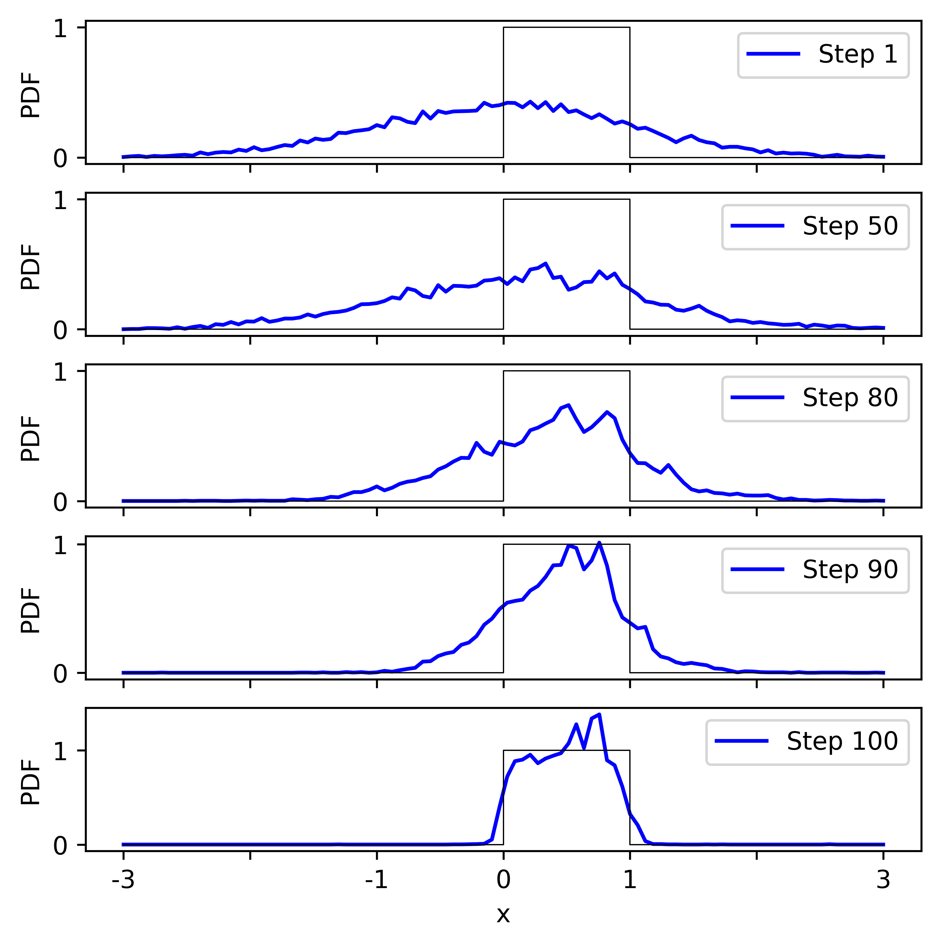
We generate 10000 samples using the trained DM, and store the intermediate steps.
- The plot shows histograms of samples.
- The initial distribution, at Step 1, is unit Gaussian.
- Effect of noise becomes discernible around Step 50.
- Gradually the distribution becomes closer to $U[0,1]$.
- It is not perfect - we will refine the model later.
What is an SDE
Consider a generic SDE $$ dx = f(x,t)dt + g(x,t)dw $$ where
- $x\in\bR^n$ is the states;
- $f(x,t):\bR^n\times \bR^+\mapsto\bR^n$ is the dynamics, or the drift in SDE;
- $w\in\bR^n$ is noise that follows a "Wiener process" - think it as Gaussian at every time step;
- $g(x,t):\bR^n\times \bR^+\mapsto\bR^{n\times n}$ is the diffusion in SDE, that governs the strength of noise.
Example 1D SDE
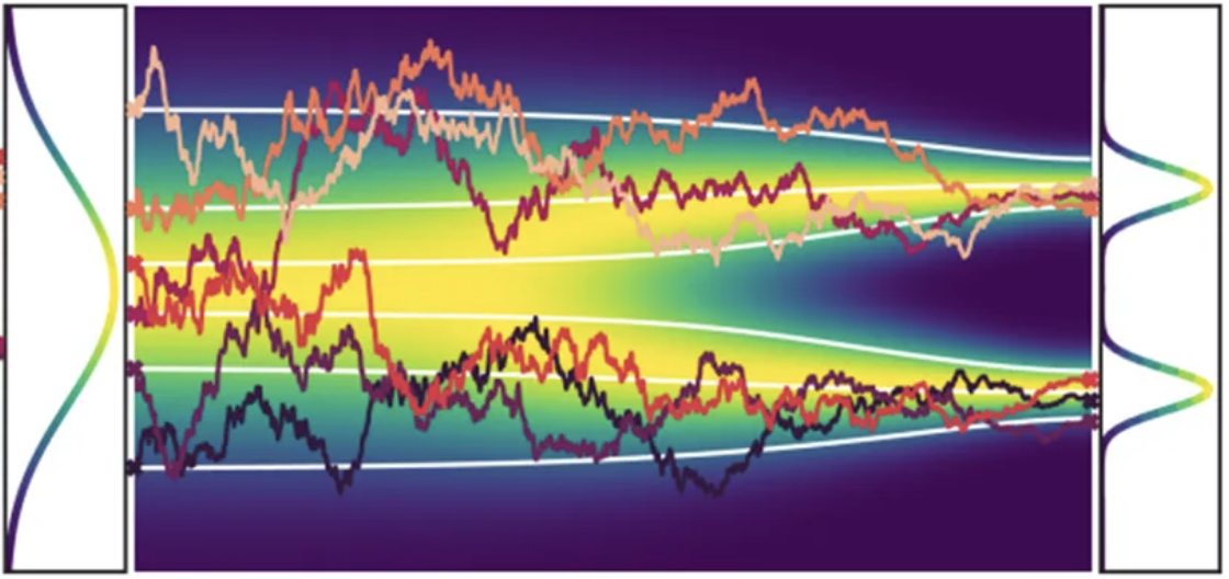
(medium.com/@ninadchaphekar)
- One noisy curve is one SDE solution, say, from $0$ to $T$
- The drift controls the average trend of the solution; the diffusion controls the amount of noise
- If we sample a lot of SDE solutions
- At every time instance $t$, $x(t)$ forms a distribution $p_t(x)$, shown in color map
- Think SDE as mapping the initial time distribution $p_0(x)$ to end time distribution $p_T(x)$
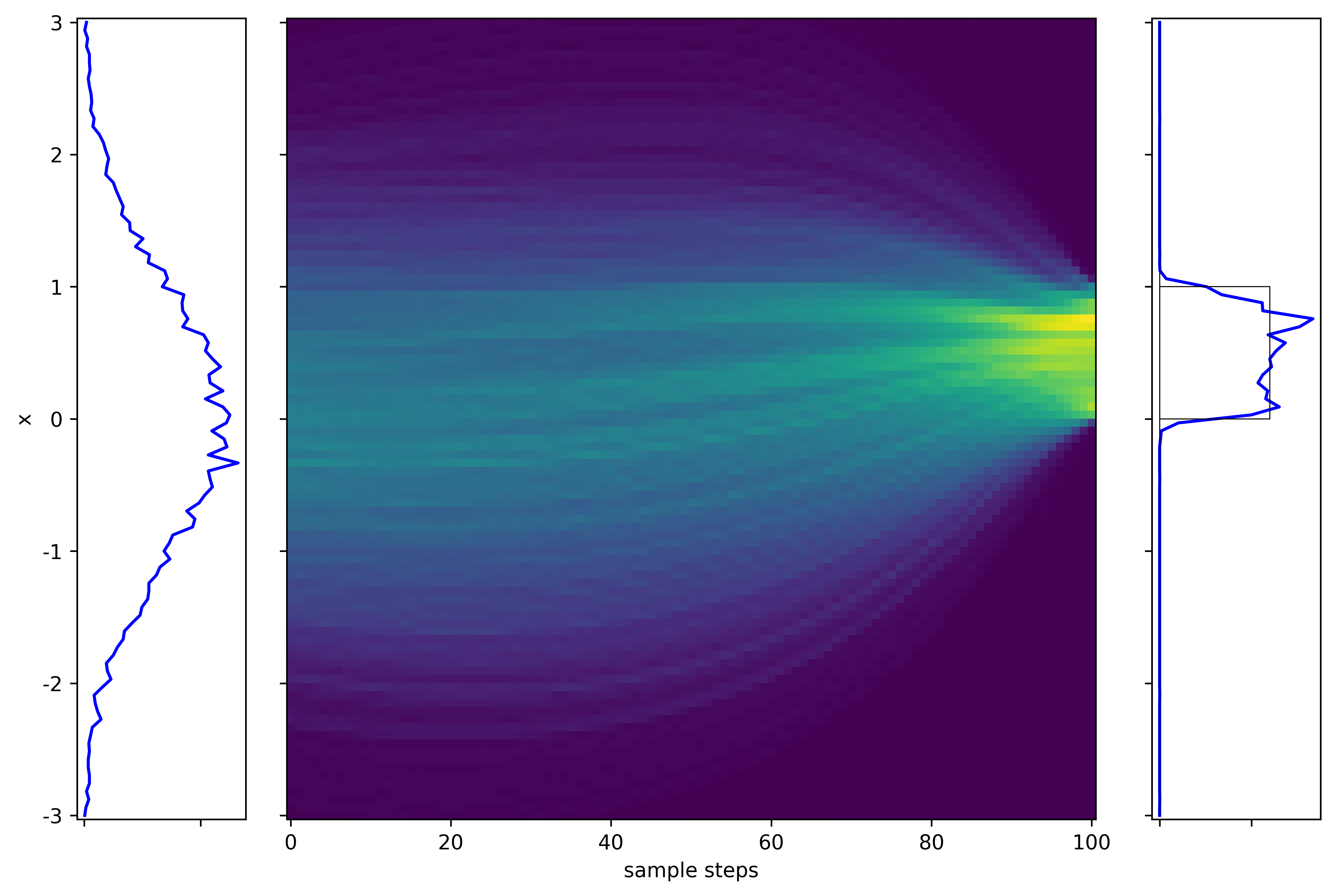
In the earlier numerical example, the corresponding color map is the following.
We see how Gaussian distribution evolves into $U[0,1]$.
Discretization of SDE
The SDE is effectively taking the limit, $\Dt\rightarrow 0$, of the following, $$ x(t+\Dt)-x(t) = f(x,t)\Dt + g(x,t)\sqrt{\Dt}\epsilon,\quad \epsilon\sim N(0,I) $$
- It is as if forward Euler scheme for an ODE
- But with Gaussian noise added at every time step
The factor $\sqrt{\Dt}$ is to ensure the equal contribution of drift and diffusion to the variance.
SDEs in DM
 (medium.com/@ninadchaphekar)
- The encoder and decoder are represented using SDEs (forward and reverse)
- We will see that DM only needs to learn a part of the reverse SDE
- The "probability flow ODE" will be discussed later.
Forward SDE
Consider a simplified SDE with scalar $g(t)$ $$ dx = f(x,t)dt + g(t)dw $$
For simplicity, we will denote $$ x(t)\equiv x_t,\ x(t+k\Dt)\equiv x_{t+k} $$ Similarly $f(x,t)\equiv f_t$, $g(x,t)\equiv g_t$, and the discretization is $$ x_{t+1}-x_t = f_t\Dt + g_t\sqrt{\Dt}\epsilon,\quad \epsilon\sim N(0,I) $$
Using the discretized form, from properties of Gaussian distribution, $$ p(x_{t+1}|x_t) = N(x_t + f_t\Dt, g_t^2\Dt I) $$ where
- The mean is as if the "deterministic" part of dynamics.
- The covariance is proportional to $\Dt$, which somewhat explains the earlier choice of $\sqrt{\Dt}$.
- The probability is a function of both $x$ and $t$.
We have seen something very similar in the Bayesian formulation!
Reverse/Backward SDE
Given the form of forward SDE, the reverse is $$ dx = \left[ f_t - g_t^2\nabla_x\log p_t(x) \right]dt + g_tdw $$
The new term in backward SDE is called the score function in the literature, denote $$ s(x,t) = \nabla_x\log p_t(x) $$
The name is due to another context. Here it is really just the gradient of the log of a PDF.
If $s(x,t)$ is known, then we can solve the backward SDE to revert the process of forward SDE.
- Forward SDE adds noise to produce Gaussian noise.
- Backward SDE "removes" noise to recover the original distribution.
EXTRA -->
Derivation of backward SDE
For ease of notation, let $t=0$.
From the forward Gaussian distribution $$ p(x_1|x_0)\propto \exp\left( -\frac{\norm{x_1-x_0-f_0\Dt}^2}{2g_0^2\Dt} \right) $$
To obtain the backward SDE, we will revert the discretization process: First find $p(x_0|x_1)$, then take limits $\Dt\rightarrow 0$.
Using Bayes theorem, $$ \begin{align*} p(x_0|x_1) &= \frac{p(x_1|x_0)p(x_0)}{p(x_1)} = p(x_1|x_0)\exp(\log p(x_0) - \log p(x_1)) \\ &\propto \exp\left( -\frac{\norm{x_1-x_0-f_0\Dt}^2}{2g_0^2\Dt} + \log p(x_0) - \log p(x_1) \right) \end{align*} $$
Consider Taylor series expansion, $$ \log p(x_1) = \log p(x_0) + (x_1-x_0)\cdot\nabla_x\log p(x_0) + \Dt \frac{\partial}{\partial t}\log p(x_0) $$ The exponential simplifies as $$ p(x_0|x_1) \propto \exp\left( -\frac{\norm{x_1-x_0-f_0\Dt}^2}{2g_0^2\Dt} - (x_1-x_0)\cdot\nabla_x\log p(x_0) + O(\Dt) \right) $$
By completion of squares, $$ p(x_0|x_1) \propto \exp\left( -\frac{\norm{x_1-x_0-(f_0-g_0^2\nabla_x\log p(x_0))\Dt}^2}{2g_0^2\Dt} + O(\Dt) \right) $$ and up to a difference of $O(\Dt)$ $$ p(x_0|x_1) \propto \exp\left( -\frac{\norm{x_0-x_1+(f_1-g_1^2\nabla_x\log p(x_1))\Dt}^2}{2g_1^2\Dt} + O(\Dt) \right) $$
As $\Dt\rightarrow 0$, $$ p(x_0|x_1) = N(x_1 - (f_1-g_1^2\nabla_x\log p(x_1))\Dt, g_1^2\Dt I) $$ which corresponds to the backward SDE $$ dx = \left[ f(x(t)) - g(t)^2\nabla_x\log p(x(t)) \right]dt + g(t)dw $$
<-- EXTRA
Score function
The DM would be fully determined once we know $$ s(x,t) = \nabla_x\log p(x(t)) $$
To do so, we can try to compute $p_t(x)\equiv p(x(t))$.
EXTRA -->
Say we solve forward SDE for time $t$. Formally, given an initial condition $x_0$, the solution is $p(x_t|x_0)$.
$$ p_t(x) = \int p(x_t|x_0)p(x_0) dx_0 = \bE_{x_0}[p(x_t|x_0)] $$Then, $$ s(x,t) = \nabla_x \log p(x_t) = \nabla_x \log \bE_{x_0}[p(x_t|x_0)] = \frac{\nabla_x \bE_{x_0}[p(x_t|x_0)]}{\bE_{x_0}[p(x_t|x_0)]} = \frac{\bE_{x_0}[\nabla_x p(x_t|x_0)]}{\bE_{x_0}[p(x_t|x_0)]} $$ where the last step swaps the order of derivative and integral.
Furthermore, since $\nabla_x\log p(x)=[\nabla_x p(x)] / p(x)$ $$ s(x,t) = \frac{\bE_{x_0}[p(x_t|x_0)\nabla_x \log p(x_t|x_0)]}{\bE_{x_0}[p(x_t|x_0)]} = \int \frac{p(x_t,x_0)}{p(x_t)} \nabla_x \log p(x_t|x_0) dx_0 $$
<-- EXTRA
This would give us $$ s(x,t) = \bE_{x_0\sim q} [\nabla_x \log p(x_t|x_0)\ |\ x_t] $$ where $q(x_0|x_t)={p(x_t,x_0)}/{p(x_t)}$.
Unfortunately, the formulation is computationally intractable:
- Computing $\bE_{x_0\sim q}$ needs to loop over all $x_0$'s in dataset.
- For every $x_0$, we need to evaluate $p(x_t|x_0)$.
Both $\bE_{x_0\sim q}$ and $p(x_t|x_0)$ are expensive to evaluate!
Score matching
We first solve the issue of computing $\bE_{x_0\sim q}$.
Idea is simple: directly learn a parametrized model $s_\theta(x,t)$ to replace $\bE_{x_0\sim q}$.
EXTRA -->
A trick to use here is an identity $$ \mu=\bE[v] \quad\Leftrightarrow\quad \bE[v]=\arg\min_\mu \bE_v[\norm{\mu-v}^2] $$ which essentially says the mean $\mu$ is a value that minimizes the moment $\norm{\mu-v}^2$.
For a given $x_N$, let $\mu=s_\theta(x_t,t)$, $v=\nabla_x \log p(x_t|x_0)$
Then $s(x_t,t)$ is the minimizer of $$ \bE_{x_0\sim q} \left[ \norm{s_\theta(x_t,t) - \nabla_x \log p(x_t|x_0)}^2 \ |\ x_t \right] $$
Lastly, for $s$ to be the minimizer of any $x_t$, we need $$ \min_\theta \bE_{x_t}\left[ \bE_{x_0\sim q} \left[ \norm{s_\theta(x_t,t) - \nabla_x \log p(x_t|x_0)}^2 \ |\ x_t \right] \right] $$
Writing out the expectations explicitly, we are minimizing $$ \int\left\{\int \frac{p(x_t,x_0)}{p(x_t)} \norm{s_\theta(x_t,t)-\nabla_x \log p(x_t|x_0)}^2 dx_0\right\} dx_t $$
$p(x_t)$ is mainly a normalizing factor and can be ignored, then the objective function becomes $$ \iint p(x_t,x_0) \norm{s_\theta(x_t,t)-\nabla_x \log p(x_t|x_0)}^2 dx_0 dx_t = \bE_{x_0,x_t}\left[ \norm{s_\theta(x_t,t)-\nabla_x \log p(x_t|x_0)}^2 \right] $$
<-- EXTRA
Accounting for the sampling over interval $[0,T]$, the loss for learning $s_\theta$ is $$ \bE_{x_0,x_t,t}\left[ \norm{s_\theta(x_t,t)-\nabla_x \log p(x_t|x_0)}^2 \right] $$
Furthermore, since $p(x_t|x_0)$ is Gaussian $$ \nabla_x\log p(x_t|x_0) = -\frac{x_t-\alpha_t x_0}{\beta_t^2} = -\frac{\epsilon_t}{\beta_t} $$ If we define $$ s_\theta = -\frac{\epsilon_\theta}{\beta_t} $$ The loss from discretized version is recovered, $$ \bE_{x_0,\epsilon,t}\left[ \lambda(t)\norm{ \epsilon - \epsilon_\theta\left(\alpha_t x_0 + \beta_t \epsilon\right) }^2 \right] $$
Analytical SDE solutions
Next we solve the issue that $p(x_t|x_0)$ is difficult to compute.
- By brutal force, we need to sample many SDE solutions from an initial condition $x_0$, from which we estimate $p(x_t|x_0)$.
- In DM, we have the freedom to design $f$ and $g$ in forward SDE.
- How about we design the SDE so that $p(x_t|x_0)$ can be computed analytically?
One way to do so is "reserve engineering".
We start with a simple target PDF, say, $$ p(x_t|x_0) = N(\alpha_t x_0, \beta_t^2 I) $$ where $\alpha_t, \beta_t$ are chosen by user.
Then assume a sufficiently simple SDE, say $$ dx = f(t)xdt + g(t)dw $$ where $f$ and $g$ are scalars.
All we need is to find $f$ and $g$ so that the SDE produces the target PDF $p(x_t|x_0)$
Different choice of PDF (i.e., $\alpha_t, \beta_t$) certainly results in different SDE's and hence different DM's.
EXTRA -->
Solution procedure
We take the following strategy
- Establish recursive relations between $\alpha_k,\beta_k$ and $\alpha_{k+1},\beta_{k+1}$ from SDE,
- which contains $f_k, g_k$.
- Solve for the explicit expressions of $\alpha_t, \beta_t$.
- Solve for $f(t),g(t)$ as a function(al) of $\alpha_t, \beta_t$.
To obtain the recursive relation, note the following identity, $$ p(x_{k+1}|x_0) = \int p(x_{k+1}|x_k) p(x_k|x_0) dx_k $$
To simplify the expression above, recall the well-known identities of Gaussian distribution: If $$ p(x,y) = N\left( \begin{bmatrix}\mu_x \\ \mu_y\end{bmatrix}, \begin{bmatrix} \Sigma_{xx} & \Sigma_{xy} \\ \Sigma_{xy} & \Sigma_{yy} \end{bmatrix} \right) $$ then $$ \begin{align} p(y) &= N(\mu_y, \Sigma_{yy}) \\ p(x|y) &= N\left(\mu_x+\Sigma_{xy}\Sigma_{yy}^{-1}(y-\mu_y), \Sigma_{xx}-\Sigma_{xy}\Sigma_{yy}^{-1}\Sigma_{yx}\right) \\ p(x) &= \int p(x|y)p(y) dy = N(\mu_x, \Sigma_{xx}) \end{align} $$
In our case, $$ \begin{equation} \begin{array}{lllll} \mbox{We know} &\ p(y) &\Rightarrow p(x_k|x_0) &= N(\alpha_k x_0,\beta_k^2I) &\mbox{By definition} \\ &\ p(x|y) &\Rightarrow p(x_{k+1}|x_k) &= N(x_k+f_k x_k\Dt, g_k^2\Dt I) &\mbox{By SDE discretization} \\ \mbox{Want to know} &\ p(x) &\Rightarrow p(x_{k+1}|x_0) &= N(\alpha_{k+1}x_0,\beta_{k+1}^2I) &\mbox{By definition} \end{array} \end{equation} $$
Matching the means and variances leads to a system of equations $$ \begin{gather*} \mu_y = \alpha_k x_0,\quad \Sigma_{yy} = \beta_k^2 I,\quad \mu_x = \alpha_{k+1} x_0,\quad \Sigma_{xx} = \beta_{k+1}^2 I \\ \mu_x+\Sigma_{xy}\Sigma_{yy}^{-1}(y-\mu_y)=(1+f_k\Dt)x_k,\quad \Sigma_{xx}-\Sigma_{xy}\Sigma_{yy}^{-1}\Sigma_{yx}=g_k^2\Dt I \end{gather*} $$
Condensing into two equations, with $y=x_k$ $$ \begin{align*} \alpha_{k+1} x_0 + \beta_k^{-2}\Sigma_{xy}(x_k-\alpha_k x_0) &= (1+f_k\Dt)x_k \\ \beta_{k+1}^2 I - \beta_k^{-2}\Sigma_{xy}\Sigma_{yx} &= g_k^2\Dt I \end{align*} $$
$p(x_{k+1}|x_0)$ should depend only on $x_0$ and not on $x_k$. Hence we must have $$ \Sigma_{xy} = \beta_k^2(1+f_k\Dt) $$ Then the recursive relations are obtained as follows $$ \begin{align*} \alpha_{k+1} x_0 = \beta_k^{-2}\Sigma_{xy}\alpha_k x_0 &\Rightarrow \alpha_{k+1} = (1+f_k\Dt)\alpha_k \\ \beta_{k+1}^2 I = \beta_k^{-2}\Sigma_{xy}\Sigma_{yx} + g_k^2\Dt I &\Rightarrow \beta_{k+1}^2 = \beta_k^2(1+f_k\Dt)^2 + g_k^2\Dt \end{align*} $$
Next we solve for the recursive relations. Knowing $\Dt\rightarrow 0$, we ignore all $O(\Dt^2)$ terms.
Using Taylor series expansion, we find the governing equations for $\alpha$ and $\beta$, $$ \begin{align*} \alpha_k + \dot{\alpha}_k \Dt &= (1+f_k\Dt)\alpha_k \\ \Rightarrow \dot{\alpha}_k &= f_k\alpha_k \\ \beta_k^2 + \dot{(\beta_k^2)} \Dt &= \beta_k^2(1+2f_k\Dt) + g_k^2\Dt \\ \Rightarrow \dot{(\beta_k^2)} &= 2f_k\beta_k^2 + g_k^2 \end{align*} $$ where $\dot{\Box}=\frac{d\Box}{dt}$.
<-- EXTRA
After some simplification, we find $f$ and $g$, $$ f(t) = \frac{\dot{\alpha_t}}{\alpha_t},\quad g(t)^2 = \alpha_t^2 \frac{d}{dt}\frac{\beta_t^2}{\alpha_t^2} $$ Next we examine a few examples.
Variance-Preserving (VP) SDE
Over $N$ steps, suppose we want the mean to evolve from $x_0$ to $0$, $$ \alpha_0=1,\ \alpha_N\approx 0 $$ and the variance to evolve from $0$ to identity, $$ \beta_0=0,\ \beta_N\approx 1 $$
For any $\alpha_t$ that satisfies the conditions, we can choose $\beta_t^2=1-\alpha_t^2$ to satisfy the other conditions.
One particular instance is, $$ \alpha_t = \exp(-t),\quad \beta_t = \sqrt{1-\exp(-2t)} $$ which produces a very simple SDE $$ f(t) = -1,\quad g(t) = 2 $$ and corresponds to a forward process of $$ x_{t+1} = (1-\Dt)x_t + 2\sqrt{\Dt}\epsilon_t $$
Another instance of VP SDE is actually the DDPM. Given $b_\max,b_\min$, let $$ a(t) = \exp\left(\frac{1}{2}b_d t^2+b_\min t\right),\quad b(t) = b_d t+b_\min,\quad b_d=b_\max-b_\min $$ and $$ \alpha_t = \sqrt{a(t)},\quad \beta_t = \sqrt{1-a(t)} $$ The SDE is $$ f(t) = -\frac{1}{2} b(t),\quad g(t) = \sqrt{b(t)} $$ The equivalent forward process is $$ x_{t+1} = \sqrt{1-b(t)}x_t + \sqrt{b(t)}\epsilon_t $$
Variance-Exploding (VE) SDE
Alternatively, we could design $\beta_t$ to grow unbounded.
This way we cover a large latent space that could be sampled from.
An instance of VE SDE is called "Score matching with Langevin dynamics (SMLD)".
Given any growth of $\sigma^2(t)$, $$ \alpha_t=1,\quad \beta_t=\sigma^2(t) $$ The SDE is $$ f(t)=0,\quad g(t)=\sqrt{\frac{d\sigma^2}{dt}} $$ The equivalent forward process is $$ x_{t+1} = x_t + \sqrt{\sigma_{t+1}^2-\sigma_t^2}\epsilon_t $$
A simple example is to assume a linear growth of variance $\sigma^2(t)=t$, which corresponds to $$ f(t)=0,\quad g(t) = 2t $$
Probability Flow ODE
Consider the SDE $$ dx = f(x,t)dt + g(t)dw $$
The following "probability flow ODE" generates the same distribution as the SDE $$ \dot{x} = f(x,t) - \frac{1}{2} g(t)^2\nabla_x \log p(x) $$
Furthermore, reserve process of the ODE is itself.
- $\nabla_x \log p(x)$ is the score function, represented by a neural network.
- $f(x)$ and $g(t)$ are chosen by user.
- Hence the ODE is a neural ODE, for which many learning algorithms exist. $$ \dot{x} = f(x) - \frac{1}{2}g(t)^2 s_\theta(x,t) $$
- Once we learned $s_\theta(x,t)$, the ODE is solved to generate new data.
For example, for the earlier numerical example, we essentially learned an ODE with the following vector field
See how the vector, i.e., $\dot{x}$, drives the Gaussian (left) to $U[0,1]$ (right).
EXTRA -->
Derivation
From the SDE $$ dx = f(x,t)dt + g(t)dw $$ The evolution of $p(x)$ satisfies the Fokker-Planck (FP) equation, $$ \frac{\partial}{\partial t} p(x) = - \nabla_x\cdot[p(x)f(x)] + \frac{1}{2} g(t)^2\nabla_x^2 p(x) $$ where note again we assume $g(t)$ is a scalar.
Now factor the RHS by a scalar $\sigma(t)\leq g(t)$, $$ \begin{align*} \frac{\partial}{\partial t} p(x) &= - \nabla_x\cdot[p(x)f(x)] + \frac{1}{2} g(t)^2\nabla_x^2 p(x) \\ &= - \nabla_x\cdot\left[p(x)f(x) + \frac{1}{2} \left(\sigma(t)^2-g(t)^2\right)\nabla_x p(x) \right] + \frac{1}{2} \sigma(t)^2\nabla_x^2 p(x) \end{align*} $$
Note the identity $$ \nabla_x p(x) \equiv \left(\nabla_x \log p(x)\right) p(x) $$ The FP equation transforms into $$ \frac{\partial}{\partial t} p(x) = - \nabla_x\cdot\left[p(x) \left(f(x) + \frac{1}{2} \left(\sigma(t)^2-g(t)^2\right)\nabla_x \log p(x) \right)\right] + \frac{1}{2} \sigma(t)^2\nabla_x^2 p(x) $$
Score function shows up again!
The FP equation corresponds to an SDE $$ dx = \left(f(x) - \frac{1}{2} \left(g(t)^2-\sigma(t)^2\right)\nabla_x \log p(x) \right) dt + \sigma(t)dw $$
It is trivial to derive the backward version $$ dx = \left(f(x) - \frac{1}{2} \left(g(t)^2+\sigma(t)^2\right)\nabla_x \log p(x) \right) dt + \sigma(t)dw $$
The key takeaway is that,
- There are infinitely many SDEs that produce the same $p(x)$ as the original SDE.
Choosing the special case $\sigma(t)=0$, we obtain a deterministic ODE, $$ \dot{x} = f(x) - \frac{1}{2} g(t)^2\nabla_x \log p(x) $$ whose reserve process is itself.
<-- EXTRA
Design Space of DM
We follow the EDM paper to present a unified framework of a variety of DMs.
See the appendix of the paper for derivation details.
Parametrization of SDE
We consider $f(x,t)\equiv f(t)x$, so the SDE $$ dx = f(t)xdt + g(t)dw $$
We hope to design the terms in SDE such that $$ x_t = s_t x_0 + s_t\sigma_t \epsilon,\quad \epsilon\sim N(0,I) $$
Following earlier derivation, the two forms are related by $$ f(t) = \frac{\dot{s}_t}{s_t},\quad g(t) = s_t\sqrt{2\dot{\sigma}_t\sigma_t} $$
Parametrization of ODE
The probability $$ p(x_t,t) = s_t^{-d} p(x_t/s_t,\sigma_t) $$ where $d=\mathrm{dim}(x)$
With $f$, $g$, $p$ expressed in $s$ amd $\sigma$, the ODE becomes $$ dx = \left[ \frac{\dot{s}_t}{s_t}x - s_t^2\dot{\sigma}_t\sigma_t\nabla_x\log p\left(\frac{x_t}{s_t},\sigma_t\right) \right]dt $$
So effectively $d(\sigma_t^2)$ is our new time variable.
Parametrization of Loss
Due to the reparameterization, the loss is simplified a bit as $$ \bE_{x_0,\epsilon}\norm{x_0-\epsilon_\theta(x_0+\epsilon,\sigma)}^2 $$ and the score function $$ \nabla_x\log p(x,\sigma) = \frac{\epsilon_\theta(x,\sigma)-x}{\sigma^2} $$
This further simplifies the PF ODE, $$ dx = \left[ \left(\frac{\dot{\sigma}_t}{\sigma_t}+\frac{\dot{s}_t}{s_t}\right)x - \frac{\dot{\sigma}_t s_t}{\sigma_t}\epsilon_\theta\left(\frac{x}{s_t},\sigma_t\right) \right] dt $$
Parametrization of Score function/Denoiser
For easier training of $\epsilon_\theta$, one can design its structure and scale its inputs and outputs.
One choice is $$ \epsilon_\theta(x,\sigma) = c_s(\sigma)x + c_o(\sigma)F_\theta(c_i(\sigma)x,c_n(\sigma)) $$ where
- $F_\theta$ is the NN to be learned
- $c_s$ adds a skip connection term
- $c_i$ and $c_o$ scale inputs and outputs, respectively
- $c_n$ is scaled noise
After this step, common DM variants can all be written under this framework.
 (The EDM paper)
Numerical Example
First we revisit the Gaussian to $U[0,1]$ example with different DMs.
We start with comparing the "flow" field.
- Exploding formulations sample from a much more spreadout region
- EDM converges quicker and more accurately to the target distribution
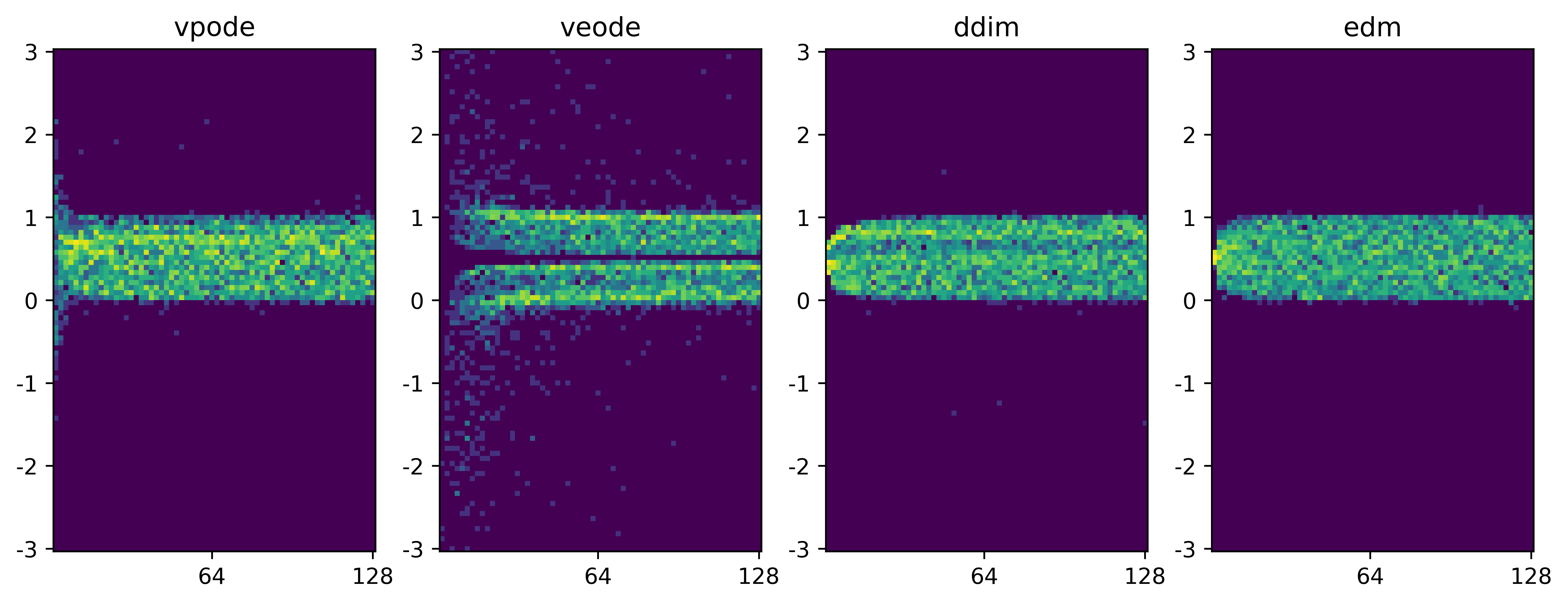
We also examine the impact of number of steps, $N$, on the sampling performance.
- All DMs are trained assuming 100 noise injection steps
- Due to the ODE formulation, we can easily change $N$ in sample generation
- This results in a trade-off between sampling accuracy and computational cost.
- $x$-axis shows $N$, color map shows the distribution of generated samples for different $N$.
- All DMs produce reasonable $U[0,1]$ when $N$ is high (to the right of x-axis)
- EDM appears to be the most robust one even with a small $N$.
Lastly, we show also a different example
- A DM that generates samples on a torus; EDM is used.
- It maps 3D Gaussian to points on a 2D surface - note here is also a flavor of dimension reduction.