$$ \newcommand\norm[1]{{\left\lVert #1 \right\rVert}} \newcommand{\bE}{\mathbb{E}} \newcommand{\bR}{\mathbb{R}} \newcommand{\vf}{\mathbf{f}} \newcommand{\vtf}{\boldsymbol{\phi}} \newcommand{\Dt}{\Delta t} $$
TODAY: Diffusion Models (DMs)
- Conditioned version, i.e., DM with inputs
References:
- References in slides
Before you move on, please make sure you have gone through the slides on the unconditioned version.
The missing piece
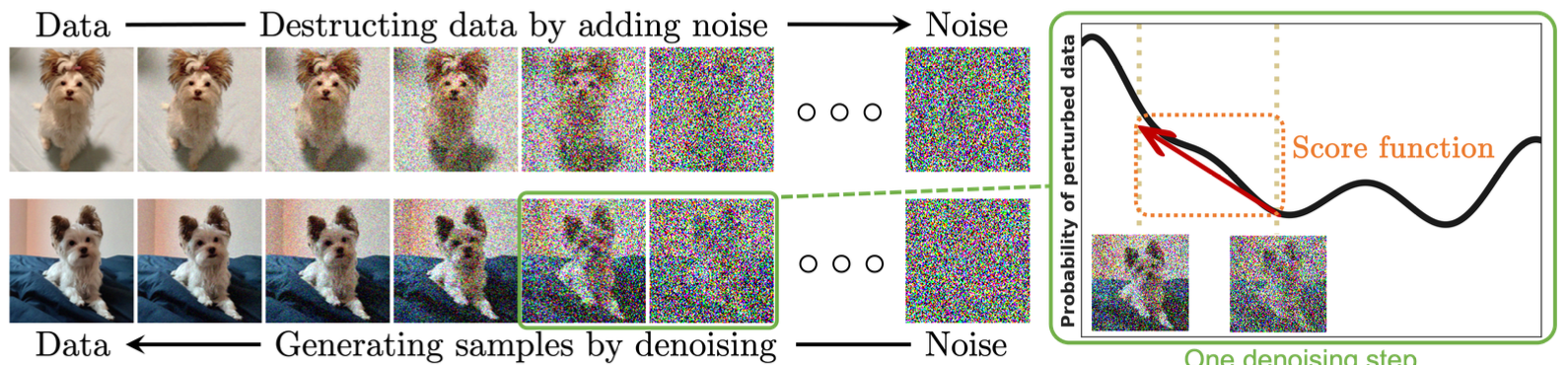 (Figure from Yang2024)
- We have discussed the forward and backwawrd processes in DM
- Via perspectives of Markov chain, SDE, and ODE.
- But we don't have control on the output
- e.g., if a DM generates images of animals, how to instruct it to generate cat images only?
To be accurate,
- Now we know how to sample $p(x)$ by solving $$ \dot{x} = f(x,t) - \frac{1}{2} g(t)^2 \underbrace{\nabla_x \log p(x)}_{\equiv s(x;\theta)} \equiv f(x,t) + \frac{1}{2} \tilde{g}(t)^2 \epsilon(x;\theta) $$
- How to sample $p(x|y)$, $y$ as the label?
- Tricky aspect: $p(x|y)$ is a different distribution from $p(x)$.
- You might guess - need to do something on $s(x;\theta)$ and/or $\epsilon(x;\theta)$.
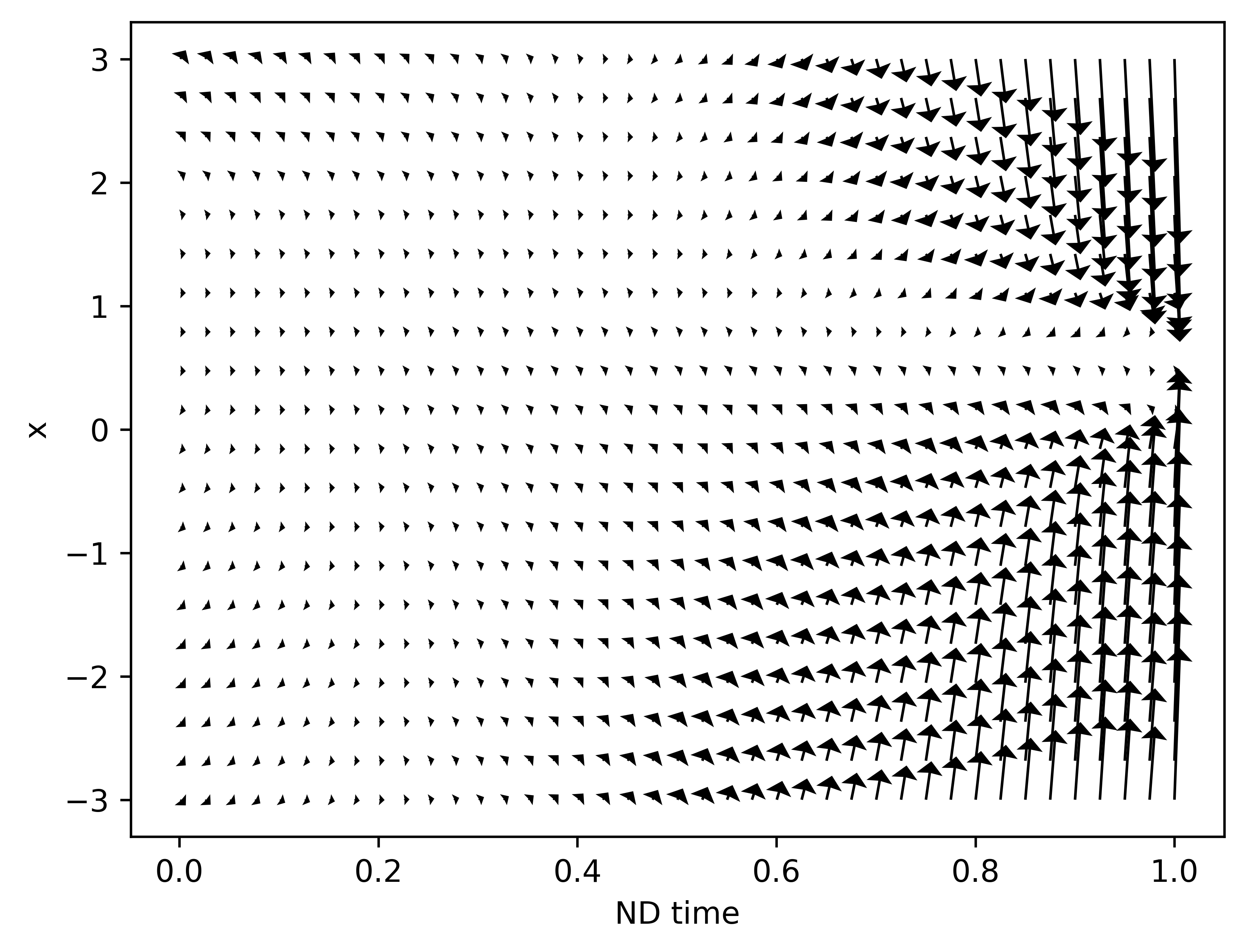
Conceptually, our previous 1D example had a vector field that drives the Gaussian (left) to $U[0,1]$ (right).
Can we modify $s(x;\theta)$ to instruct DM to drive the Gaussian to $U[0,0.5]$ or $U[0.5,1]$?
Sampler of Solutions
- Make $\epsilon(x;\theta)$ dependent on $y$ as well.
- During training. Example: Feature‑wise Linear Modulation (FiLM)
- After training. Example: Low‑Rank Adaptation (LoRA)
- Manipulate the sampling process towards the $y$ label.
- During training. Example: Classifier‑free guidance (CFG)
- After training. Example: Classifier guidance (CG)
But in practice, the above solutions can be combined.
Solution 1.1: FiLM
So we want to directly replace $\epsilon(x;\theta)$ with $\epsilon(x,y;\theta)$.
- Better to preserve the NN architecture of the original $\epsilon(x;\theta)$.
Idea of FiLM: Replace weights $W$ in $\epsilon(x;\theta)$ with $$ W' = \gamma(y)W + \beta(y) $$ where $\gamma$ and $\beta$ are small encoding networks.
Now the sampling process: $$ \dot{x} = f(x,t) + \frac{1}{2} \tilde{g}(t)^2 \epsilon(x;{\color{red}{\theta(y)}}) $$
- $y$ changes weights $\rightarrow$ vector field changes $\rightarrow$ generated sample change.
Solution 1.2: LoRA
- In FiLM, $\gamma$ and $\beta$ are trained together with $\epsilon$.
- Expensive, and inconvenient to change after training (e.g., add new labels/outputs)
- Can we use two stages:
- Pretrain a model: $\epsilon(x;\theta)$
- Modify $\theta$ for some $y$: $\epsilon(x;\theta+{\color{red}{\delta\theta(y)}})$
Idea of LoRA: Modify weights $W$ in $\epsilon(x;\theta)$ as $$ W' = W + \delta W \equiv W + AB^\top $$ with $A$ and $B$ as learnable low-rank matrices.
Low-rank matrices are
- Efficient to store: GB-level pretrained model vs MB-level LoRA modifications
- Efficient to evaluate: $$ W'x = Wx + (A{\color{red}{(B^\top x)}}) $$
The catch in LoRA:
- Given new $y$, one needs some additional training
- Potential overfit
Solution 2.1: CG
Now, some less brutal-force approach.
We want $\nabla_x \log p(x|y)$, but Bayes theorem gives $$ p(x|y) = \frac{p(y|x)p(x)}{p(y)} $$ and hence $$ \nabla_x \log p(x|y) = \underbrace{\nabla_x \log p(y|x)}_{\text{Unknown}} + \underbrace{\nabla_x \log p(x)}_{\text{Trained}} - \underbrace{\nabla_x \log p(y)}_{=0} $$
- The only unknown $p(y|x)$ is a simple classifier!
CG process:
- Starting from a trained model $s(x;\theta)$
- Train an additional classifier $p(y|x)$
- Generate new samples as $$ \begin{aligned} \dot{x} &= f(x,t) - \frac{1}{2} g(t)^2 \nabla_x \log p(x|y) \\ &= f(x,t) - \frac{1}{2} g(t)^2 \left(s(x;\theta) + \nabla_x \log p(y|x) \right) \end{aligned} $$
More refined tuning $$ \dot{x} = f(x,t) - \frac{1}{2} g(t)^2 \left(s(x;\theta) + {\color{red}\gamma}\nabla_x \log p(y|x) \right) $$
- Parameter $\gamma$: balance between relevance and diversity
- If $\gamma>1$: Closer to the labelled samples, but less diverse
The catch:
- The classifier $p(y|x)$ is used during denoising, so $x$ is noisy
- The classifier needs to handle noise robustly
- Or alternatively, use $\epsilon(x;\theta)$ to denoise first
Solution 2.2: CFG
History is a loop
After CG, some people ask: How about we directly learn $$ s(x,y;\theta) = \nabla_x \log p(x|y) $$ Then the sample generation is $$ \dot{x} = f(x,t) - \frac{1}{2} g(t)^2 \underbrace{\nabla_x \log p(x|y)}_{\Rightarrow s(x,y;\theta)} $$
To avoid modifying model architecture, apply the following tricks:
- Allow an "empty label" $\emptyset$, representing any label, so $s(x,\emptyset;\theta)$ represents the usual unconditioned score.
- Train with labelled data samples $(x,y)$, but with "low probability" drop the label, so a data sample temporarily becomes $(x,\emptyset)$.
- So $s(x,y;\theta)$ embeds all samples, and somewhat "organized" by their labels.
Furthermore, we can do refined tuning as well.
Rewrite the CG version as $$ \begin{aligned} &\quad s(x;\theta) + \gamma\nabla_x \log p(y|x) \\ &= \gamma (\underbrace{s(x;\theta) + \nabla_x \log p(y|x)}_{=\text{Conditioned score}}) + (1-\gamma)(\underbrace{s(x;\theta)}_{=\text{Unconditioned score}}) \\ &= \gamma s(x,y;\theta) + (1-\gamma) s(x,\emptyset;\theta) \end{aligned} $$
Practically, people use $w=\gamma-1$ and $$ (1+w)\epsilon(x,y;\theta) - w\epsilon(x,\emptyset;\theta) $$
Numerical Example
Consider the previous scalar example, meaning $x\in\bR$.
The training dataset consists of samples from uniform distribution over $[0,1]$, i.e., $U[0,1]$.
The DM has the following vector field that drives the Gaussian (left) to $U[0,1]$ (right).
Can we instruct DM to drive the Gaussian to $U[0,0.5]$ or $U[0.5,1]$?
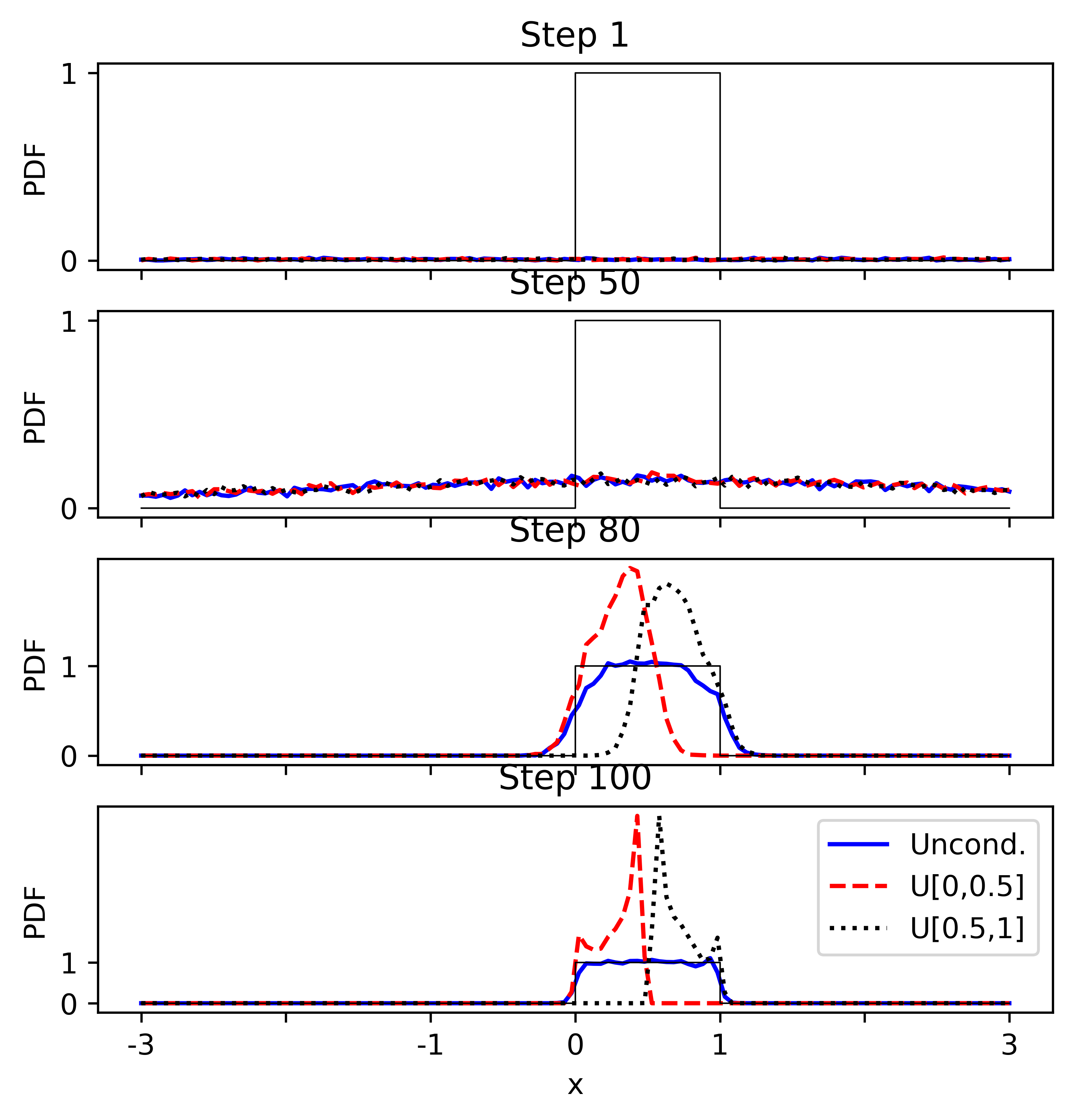
Using CFG, here are the results - did the job as expected.
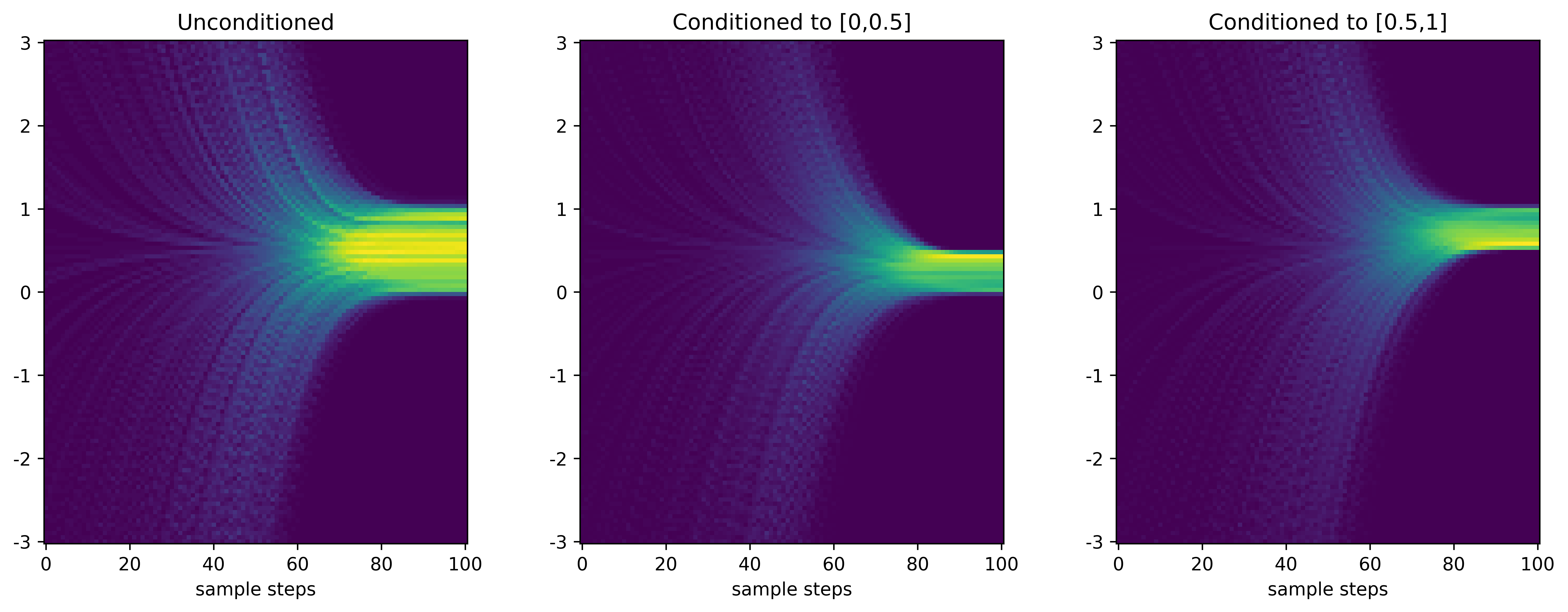
Detailed look - CFG scheduling $$ w_k = 5\left(\frac{i}{100}\right)^5,\quad k=0,1,\cdots,99 $$
- Initially not much difference; conditioning comes towards the end; distributions not that perfect though.