Machine Learning for Engineering

Dynamical System: Diffusion Models, Flow Matching

Instructor: Daning Huang

$$ \newcommand\norm[1]{{\left\lVert #1 \right\rVert}} \newcommand{\bE}{\mathbb{E}} \newcommand{\cL}{\mathcal{L}} \newcommand{\vf}{\mathbf{f}} \newcommand{\vtf}{\boldsymbol{\phi}} $$

TODAY: Diffusion Models (DMs)

• Flow matching perspective

References:

• A nice intro blog dl.heeere.com - We acknowledge the authors and used many visualizations from this article
• Liu2022
• Lipman2023
• Tong2023
• Other references in slides

Technically, this part can be learned independently from the DM slides.

Intuition of Flow Matching

Rethinking DM

Recall what a DM entails:

• A sequence of probability distributions $$p(x_0) \longleftrightarrow p(x_1) \longleftrightarrow \cdots \longleftrightarrow p(x_T)$$
  • $p(x_0)$ is easy to sample (e.g., Gaussian), and $p(x_N)$ is the target distribution

• A sequence of samples $$x_0 \longleftrightarrow x_1 \longleftrightarrow \cdots \longleftrightarrow x_T$$
  • These are solutions of an ODE/SDE/Markov process, given an initial condition $x_0$

To design a DM,

• [Probability Path] First, design the probability distributions, e.g., something like $$ p(x_t|x_0) = N(\alpha_t x_0, \beta_t^2 I) $$ where one chooses $\alpha_t$ and $\beta_t$.

• [Velocity Field] Then find the RHS of differential equation that governs the changes in $p(x)$, e.g., something like $$ \dot{x} = f_t - \frac{1}{2}g_t^2\nabla_x\log p_t(x) \equiv v_\theta(x,t) $$ where $f_t$ and $g_t$ are determined by $\alpha_t$ and $\beta_t$, and $\nabla_x\log p_t(x)$ is learnt from data.

• [Flow] Lastly, find the DE solution to generate samples $$ x_t = \psi_t(x_0) $$ where $x_0=\psi_0(x_0)$, $x_T=\psi_T(x_0)$, and $\frac{\partial\psi_t}{\partial t} = v_\theta(x,t)$.

Ultimately,

Probability path, Velocity field, and Flow are equivalent descriptions of the same (diffusion) model

Up to some technical constraints - to be discussed later.

Visualizing the equivalence

Probability path: continuously deform from $p(x_0)$ (blue, Gaussian) to $p(x_T)$ (red, arbitrary)

display(HTML(pp_html))  # Taken from the heeere blog

• Velocity field: the vectors - how particles move instantaneously
• Flow: the trajectory of a particle - a sample $x_0$ from $p(x_0)$ to a target $x_T$ in $p(x_T)$

# This example aims to transform a Gaussian (blue, left) to two Gaussians (red, right)
display(HTML(vf_html))  # Taken from the heeere blog

The complaints in DM

• Low training efficiency (need to learn the noise prediction, denoising function, or score function)
• Low sampling efficiency (need to solve a differential equation every time)

Question

• Both issues are somewhat because the vector field is highly nonlinear - difficult to learn, many steps to solve
• Can we directly design the flow in a simpler form (instead of starting from probability path)

A possible solution by FM

Let's start from the flow, $$ x_t = \psi_t(x_0),\quad t\in[0,T] $$

By definition $$ x_0=\psi_0(x_0),\quad x_T=\psi_T(x_0) $$ and we need them to follow the correct distributions $$ x_0\sim p(x_0),\quad x_T\sim p(x_T) $$

If one pick a pair $(x_0,x_T)$, the simplest possible flow is perhaps (assuming $T=1$) $$ x_t = \psi_t(x_0{\color{red}{,x_T}}) = t {\color{red}{x_T}} + (1-t)x_0 $$

This produces a vector field that appears simple $$ \dot{x} = \frac{\partial \psi_t}{\partial t} = {\color{red}{x_T}} - x_0 $$

But the ODE is somewhat ill-defined,

• Starting from $x_0$, one needs $x_T$ to compute the $\dot{x}$ to solve the ODE
• But without solving ODE, one cannot compute $x_T$!

Perhaps we can approximate the vector field by a model $$ v_\theta(x,t) = x_T - x_0 $$ by minimizing $$ \bE_{x_0,x_T}\norm{v_\theta(x,t) - (x_T - x_0)}^2 $$ or equivalently $$ \bE_{x_0,x_t}\norm{v_\theta(x,t) - \frac{x_t - x_0}{t}}^2 $$

This is essentially the Rectified Flow model [Liu2022]

The subtleties

The solution seems simple, but there are two subtle problems:

First, how to verify that the flow designed earlier produces the correct target distribution?

• For example, in $\dot{x}=x_T-x_0$, the RHS seems a "constant", meaning simple translation.
• This means uniformly translating $p(x_0)$ along $x$ axis; the shape of $p(x_t)$ is always like $p(x_0)$. [Left image]
• Then, how come we would be getting the target $p(x_T)$, that is very different from $p(x_0)$? [Right image]

(Figure from heeere)

Second, the choice of $(x_0,x_T)$ seems arbitrary, so different trajectories might intersect at the same point $(t,x_t)$

• Then the flow itself is ill-defined - at every point there are multiple possible velocity vectors.

(Figure from heeere)

Key Formulations

Addressing the two subtleties will bring us to Flow Matching.

Subtlety 1: Continuity equation

Earlier we only said that the following three are equivalent: $$ \boxed{\text{Prob. path}} \begin{array}{c} \xrightarrow{\text{Derive}} \\ \color{red}{\xleftarrow[\text{Cont. Eqn.}]{}} \end{array} \boxed{\text{Velo. field}} \begin{array}{c} \xrightarrow{\text{Solve}} \\ \xleftarrow[\text{Differentiate}]{} \end{array} \boxed{\text{Flow}} $$ But actually there is a $\color{red}{\text{constraint}}$ between Probability path and Velocity field.

At any time $t$ and states $x$, the probability $p=p(x_t)$ and the velocity field $v=v(x_t,t)$ should satisfy the Continuity equation $$ \dot{p} + \nabla\cdot(p v) = 0 $$

• $\nabla$ is short-hand for gradients w.r.t. $x$
• This guarantees the conservation of probability over time (need $\int p(x)dx=1$ at any time)

If you are familiar with fluid mechanics, this is nothing but mass conservation law

• In our context, we also have the boundary conditions: $$ \text{Initial: }p(t=0)=p(x_0),\quad \text{Target: }p(t=T)=p(x_T) $$

Example

Say for the earlier example, the probability path and the velocity field are, respectively $$ p(x_t) = N(at+b,\sigma^2),\quad \dot{x} = v(x,t) = a $$ where $a$ is a (negative) constant, so everything translates in the negative $x$ direction, starting from $b$.

• If they satisfy the continuity equation, then the velocity field does generate the probability path.

Derivation:

To make things easier, let's transform the continuity equation a bit $$ \begin{aligned} \dot{p} &= -\nabla\cdot(pv) = -\nabla p\cdot v - p\nabla\cdot v \\ \Rightarrow \dot{p}/p &= -(\nabla p/p)\cdot v - \nabla\cdot v \\ \dot{(\log p)} &= -\nabla(\log p)\cdot v - \nabla\cdot v \end{aligned} $$

Next, in this example, $\log p = -\frac{(x-at-b)^2}{2\sigma^2} + \text{const}$ and $\nabla\cdot v=0$, so $$ \begin{aligned} \dot{(\log p)} + \nabla(\log p)\cdot v + \nabla\cdot v &= \frac{\partial}{\partial t} \left(-\frac{(x-at-b)^2}{2\sigma^2}\right) + \frac{\partial}{\partial x} \left(-\frac{(x-at-b)^2}{2\sigma^2}\right) a \\ &= -\frac{-2a(x-at-b)}{2\sigma^2} + \left(-\frac{2(x-at-b)}{2\sigma^2}\right) a = 0 \end{aligned} $$

Indeed the continuity equation is satisfied!

Subtlety 2: Conditioned vs Marginal

The prev. example essentially shows the following pair satisfies the continuity equation $$ p(x_t) = N(t x_T + (1-t)x_0,\sigma^2),\quad v(x,t) = x_T-x_0 $$ where $a=x_T-x_0$ and $b=x_0$.

These are conditional, because they depend on $x_0$ and $x_T$. The accurate notations are $$ p(x_t{\color{red}{\mid x_0,x_T}}) = N(t x_T + (1-t)x_0,\sigma^2),\quad v(x,t{\color{red}{\mid x_0,x_T}}) = x_T-x_0 $$

What we really want is the marginal, $$ p(x_t)=\bE_{x_0,x_T}[p(x_t{\color{red}{\mid x_0,x_T}})] = \int p(x_t{\color{red}{\mid x_0,x_T}}) p(x_0)p(x_T)dx_0dx_T $$

Now the question is what is the correct marginal velocity field $\tilde{v}(x,t)$?

	......Probability Path......	....Vector Field....	Satisfy C.E.?
Conditional (left)	$p(x_t\mid x_0,x_T)$	$v(x,t\mid x_0,x_T)$	Yes
Marginal (right)	$p(x_t)=\mathbb{E}_{x_0,x_T}[p(x_t\mid x_0,x_T)]$	${\color{red}{\tilde{v}(x,t)}}$	${\color{red}{??}}$

(Figure from heeere)

Let's pose the question as follows:

For some latent variable $z\sim p(z)$ (e.g., $z=[x_0,x_T]$)

• If $p(x_t|z)$ and $v(x,t|z)$ satisfy the C.E.,
• What is the $\tilde{v}(x,t)$ that satisfies the C.E. with $p(x_t)$?

First assume partial derivatives and integrals can exchange order, and we get $$ \begin{aligned} \frac{\partial p}{\partial t}(x_t) &= \frac{\partial}{\partial t} \int p(x_t|z)p(z) dz = -\int \frac{\partial p}{\partial t}(x_t|z)p(z) dz \\ &= -\int \nabla\cdot\left(p(x_t|z)v(x,t|z)\right)p(z) dz = -\nabla\cdot {\color{red}{\int p(x_t|z)v(x,t|z)p(z) dz}} \end{aligned} $$

We hope to get $$ \frac{\partial p}{\partial t}(x_t) = -\nabla\cdot {\color{red}{(p(x_t)\tilde{v}(x,t))}} $$

Comparing the red parts, we get $$ \begin{aligned} \tilde{v}(x,t) &= \frac{1}{p(x_t)}\int p(x_t|z)v(x,t|z)p(z) dz = \int \frac{p(x_t|z)v(x,t|z)}{p(x_t)}p(z) dz \\ &= \bE_z\left[ \frac{p(x_t|z)v(x,t|z)}{p(x_t)} \right] \end{aligned} $$

This is the marginal velocity field that

• is independent of $x_0,x_T$, or any other $z$
• will not have multiple velocities at the same point
• can be used to generate samples of $p(x_T)$

Subtlety 2, continued: Conditional loss

Now we know the earlier loss $$ \bE_{x_0,x_t}\norm{v_\theta(x,t) - \frac{x_t - x_0}{t}}^2 $$ matches $v_\theta(x,t)$ to the conditional velocity field.

Then, how to get the marginal, $\tilde{v}_\theta(x,t)$?

Computing by the $\mathbb{E}_z$ definition is probably intractable.

Let's pose the question as follows,

For the conditional, we minimize the following, given a conditional target $u(x,t|z)$ (e.g., $(x_t-x_0)/t$) $$ \cL_{CFM} = \bE_{t,z,x_t|z} \norm{v_\theta(x,t) - u(x,t|z)}^2 $$

Ideally we want to minimize the following, given a marginal target $\tilde{u}(x,t)$ $$ \cL_{FM} = \bE_{t,x_t} \norm{\tilde{v}_\theta(x,t) - \tilde{u}(x,t)}^2 $$

How do $\cL_{CFM}$ and $\cL_{FM}$ relate?

The short answer is that they are equivalent.

Here the equivalence means $$ \nabla_\theta\cL_{CFM} = \nabla_\theta\cL_{FM} $$ so -

• The conditional $v_\theta$ learned from $\cL_{CFM}$ (easy to evaluate) is exactly the marginal $\tilde{v}_\theta$.
• No longer need the $\cL_{FM}$, which is impractical to evaluate anyways.

Due to the equivalence, we will uniformly use $v_\theta$ next.

Proof: For CFM loss $$ \cL_{CFM} = \norm{v_\theta(x,t) - u(x,t|z)}^2 = \norm{v_\theta(x,t)}^2 - 2v_\theta(x,t)^\top u(x,t|z) + \norm{u(x,t|z)}^2 $$ Assuming expectation and gradient can swap order, and the last term is independent of $\theta$ $$ \nabla_\theta \cL_{CFM} = \bE_{t,z,x_t|z} \left[\nabla_\theta \norm{v_\theta(x,t)}^2\right] - 2\bE_{t,z,x_t|z} \left[\nabla_\theta v_\theta(x,t)^\top u(x,t|z)\right] $$ Similarly, for FM loss $$ \nabla_\theta \cL_{FM} = \bE_{t,x_t} \left[\nabla_\theta \norm{v_\theta(x,t)}^2\right] - 2\bE_{t,x_t} \left[\nabla_\theta v_\theta(x,t)^\top \tilde{u}(x,t)\right] $$

Next we show that the terms in $\nabla_\theta \cL_{CFM}$ and $\nabla_\theta \cL_{FM}$ are the same. $$ \bE_{t,z,x_t|z} \left[\nabla_\theta \norm{v_\theta(x,t)}^2\right] = \bE_{t,{\color{red}{x_t}}} \left[\nabla_\theta \norm{v_\theta(x,t)}^2\right]\quad (\text{Integrand does not have }z) $$ $$ \begin{aligned} \bE_{t,z,x_t|z} \left[\nabla_\theta v_\theta(x,t)^\top u(x,t|z)\right] &= \iint \nabla_\theta v_\theta(x,t)^\top u(x,t|z) p(x_t|z)p(z) dx_tdz \\ &= \iint \nabla_\theta v_\theta(x,t)^\top \frac{u(x,t|z) p(x_t|z)p(z)}{p(x_t)}p(x_t) dx_tdz \\ &= \int \nabla_\theta v_\theta(x,t)^\top \left[\int\frac{u(x,t|z) p(x_t|z)p(z)}{p(x_t)}dz \right]p(x_t) dx_t \\ &= \int \nabla_\theta v_\theta(x,t)^\top \tilde{u}(x,t)p(x_t) dx_t \\ &= \bE_{t,{\color{red}{x_t}}} \left[\nabla_\theta v_\theta(x,t)^\top \tilde{u}(x,t)\right] \end{aligned} $$

Summary of key elements

Given $p(x_0)$ (source, easy to sample) and $p(x_T)$ (target, sample from dataset)

• Design conditional flow from $x_0\sim p(x_0)$ to $x_T\sim p(x_T)$, e.g., $x_t=tx_T+(1-t)x_0$
• Determine the conditional velocity field, e.g., $u(x,t|x_0,x_T)$
• Learn the marginal velocity field $v_\theta(x,t)$ using conditional loss $\cL_{CFM}$
• Use $v_\theta(x,t)$ to generate new samples in $p(x_T)$

In the middle, $v_\theta(x,t)$ is theoretically guaranteed to map $p(x_0)$ to $p(x_T)$ by the Continuity Equation.

Design of Flow

Now we know the basic principles, and can design any FM models as we like.

Examples of FM

First consider a generic case.

Suppose the conditional probabilities are Gaussian $$ p(x_t|z)=N(\mu_t(z),\sigma_t(z)^2) $$ for some latent variable $z$ (formally called the coupling variables)

The user gets to choose what $z$, $\mu_t$, $\sigma_t$ are.

For conciseness, on this slide we drop $z$.

Suppose along one flow $x_t = \psi_t(x_0)$, $$ \frac{x_t-\mu_t}{\sigma_t} = \frac{x_0-\mu_0}{\sigma_0}\quad \text{(Optimal transport between Gaussians)} $$

This means $$ x_t = \mu_t + \sigma_t \left( \frac{x_0-\mu_0}{\sigma_0} \right) $$

The velocity is $$ \dot{x}_t = \dot{\mu}_t + \dot{\sigma}_t \left( \frac{x_0-\mu_0}{\sigma_0} \right) = \dot{\mu}_t + \dot{\sigma}_t \left( \frac{x_t-\mu_t}{\sigma_t} \right) $$

The conditional velocity field is thus $$ v(x,t|z) = \dot{\mu}_t(z) + \frac{\dot{\sigma}_t(z)}{\sigma_0(z)}\left( x_0-\mu_0(z) \right) \quad\text{or}\quad \dot{\mu}_t(z) + \frac{\dot{\sigma}_t(z)}{\sigma_t(z)}\left( x_t-\mu_t(z) \right)\quad \text{(whichever is easier)} $$

• One can verify that the conditionals $p(x_t|z)$ and $v(x,t|z)$ satisies the C.E.
• Then the marginal $\tilde{v}(x,t)$ should produce $p(x_T)$

Rectified flow

In our motivating example, we simply chose $$ z=[x_0,x_T],\quad \mu_t(z)=tx_T + (1-t)x_0,\quad \sigma_t(z)=\sigma $$ This gives us (as seen earlier) $$ v(x,t|z) = x_T - x_0 $$

Again, the left is the conditional (used in training); the right is the marginal (used in generation)

(Figure from heeere)

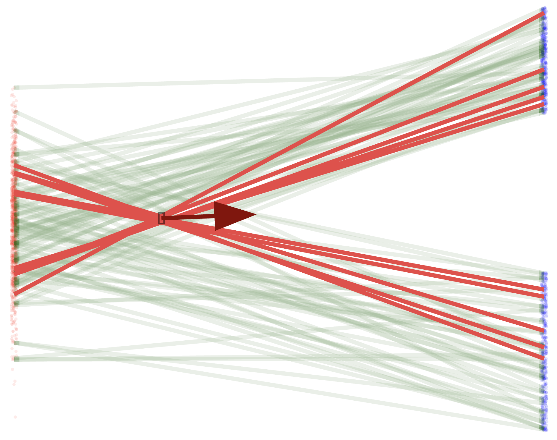
Optimal transport

OT is about transforming $p(x_0)$ to $p(x_T)$ with a minimal cost (in a certain sense).

• Theoretically the "optimal" way to do flow matching
• But extremely hard to compute, esp. for high-dim case

display(HTML(pp_html))  # Taken from the heeere blog

[Liu2022] The rectified flow provides an efficient "reflow" approach to approximate OT. Video below -

• Non-optimal: Some samples did not flow to the nearest targets - this is during the training (the conditionals)
• Sub-optimal: Most samples flow to the nearest targets, but not the shortest path - this is after training once
• Near-optimal: Most samples flow straight to the nearest targets!
  • this is a re-trained rectified flow model with the matched pairs from sub-optimal case

Video(rf_mp4)   # From authors of [Liu2022]

See also [Tong2023] for more techniques.

Connecting to diffusion models

Training

Recall one form of DM is $$ x_t = \alpha_t x_T + \sigma_t\epsilon $$

This defines a probability path that corresponds to $$ z=x_T,\quad \mu_t(z)=\alpha_tx_T,\quad \sigma_t(z)=\sigma_t $$ with user-defined $\alpha_t$ and $\sigma_t$.

Then the conditional velocity field is $$ v(x,t|z) = \frac{\dot{\sigma}_t}{\sigma_t}x + \alpha_t \left( \frac{\dot{\alpha}_t}{\alpha_t} - \frac{\dot{\sigma}_t}{\sigma_t} \right) x_T \equiv \frac{\dot{\sigma}_t}{\sigma_t}x + \sigma_t^2 \left( \frac{\dot{\alpha}_t}{\alpha_t} - \frac{\dot{\sigma}_t}{\sigma_t} \right) \underbrace{\nabla\log p(x_t)}_{\text{Score function again!}} $$

Conversely, one can also start from the ODE/SDE view of DM, $$ \dot{x} = f(t)x - \frac{1}{2}g(t)^2 s_\theta(x,t) $$ The entire RHS is the marginal velocity field!

Instead of matching the score, one can directly learn the velocity field from the conditional loss.

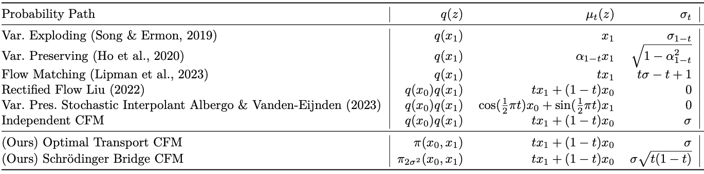
Specific instances of correspondence between FM and DMs are listed below [Tong2023]

Conditioning

We can control output given some input/label $y$, using the same techniques from DM:

In DM we manipulated the noise $\epsilon_\theta$, and now we manipulate the velocity $v_\theta$

• Make $v_\theta(x,t)$ dependent on $y$ as well.
  • During training. Example: Feature‑wise Linear Modulation (FiLM) Tong2023
  • After training. Example: Low‑Rank Adaptation (LoRA)
• Manipulate the sampling process towards the $y$ label.
  • During training. Example: Classifier‑free guidance (CFG) Zheng2023, Fan2025
  • After training. Example: Classifier guidance (CG)

A seemingly general framework: Feng2025

Examples

1D example revisited

Our previous 1D example had a vector field that drives a Gaussian to Uniform $U[0,1]$.

Let's now compare

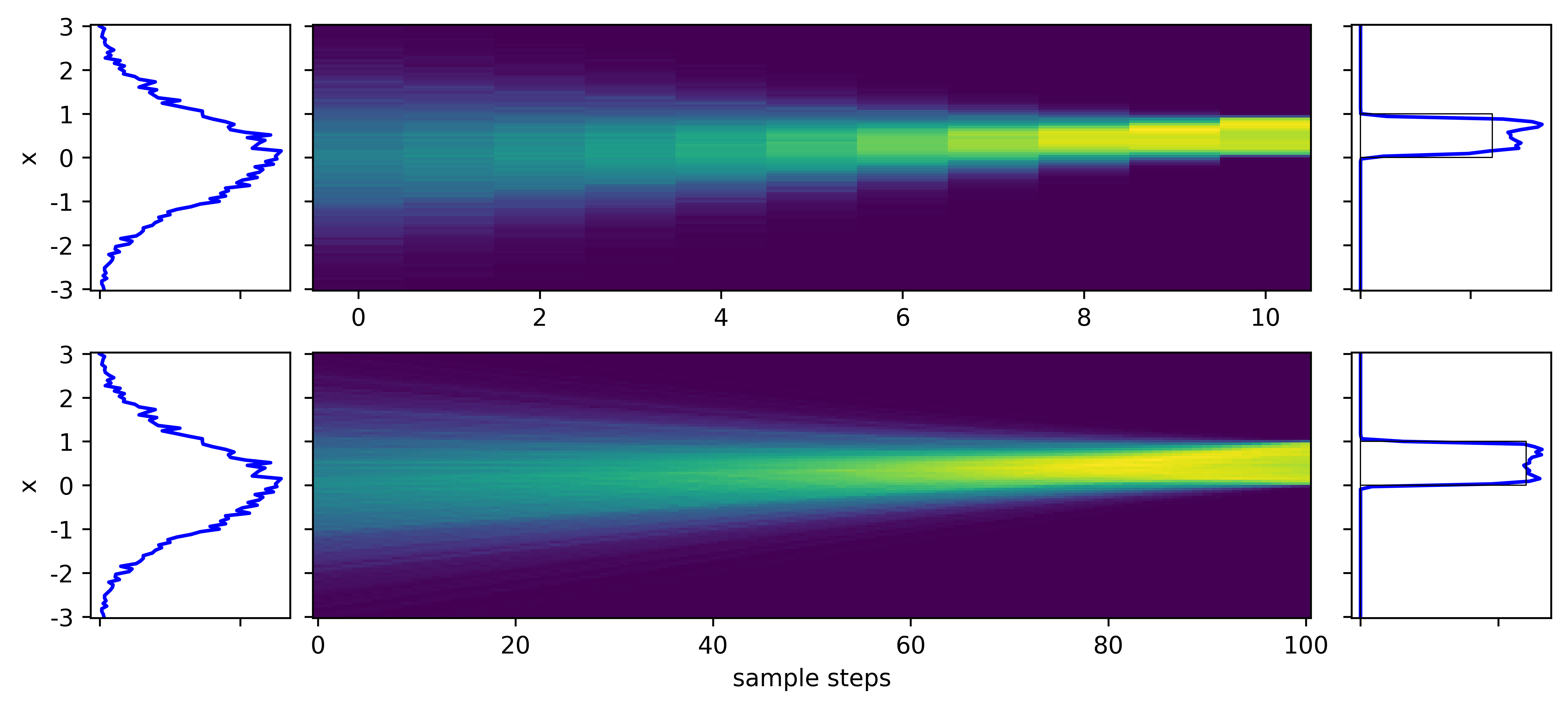
• DM, standard score matching (from prev example)
• DM, but using flow matching loss
• Pure flow matching (by rectified flow)

Note the straighter velocity fields and smoother output distributions in the FM cases

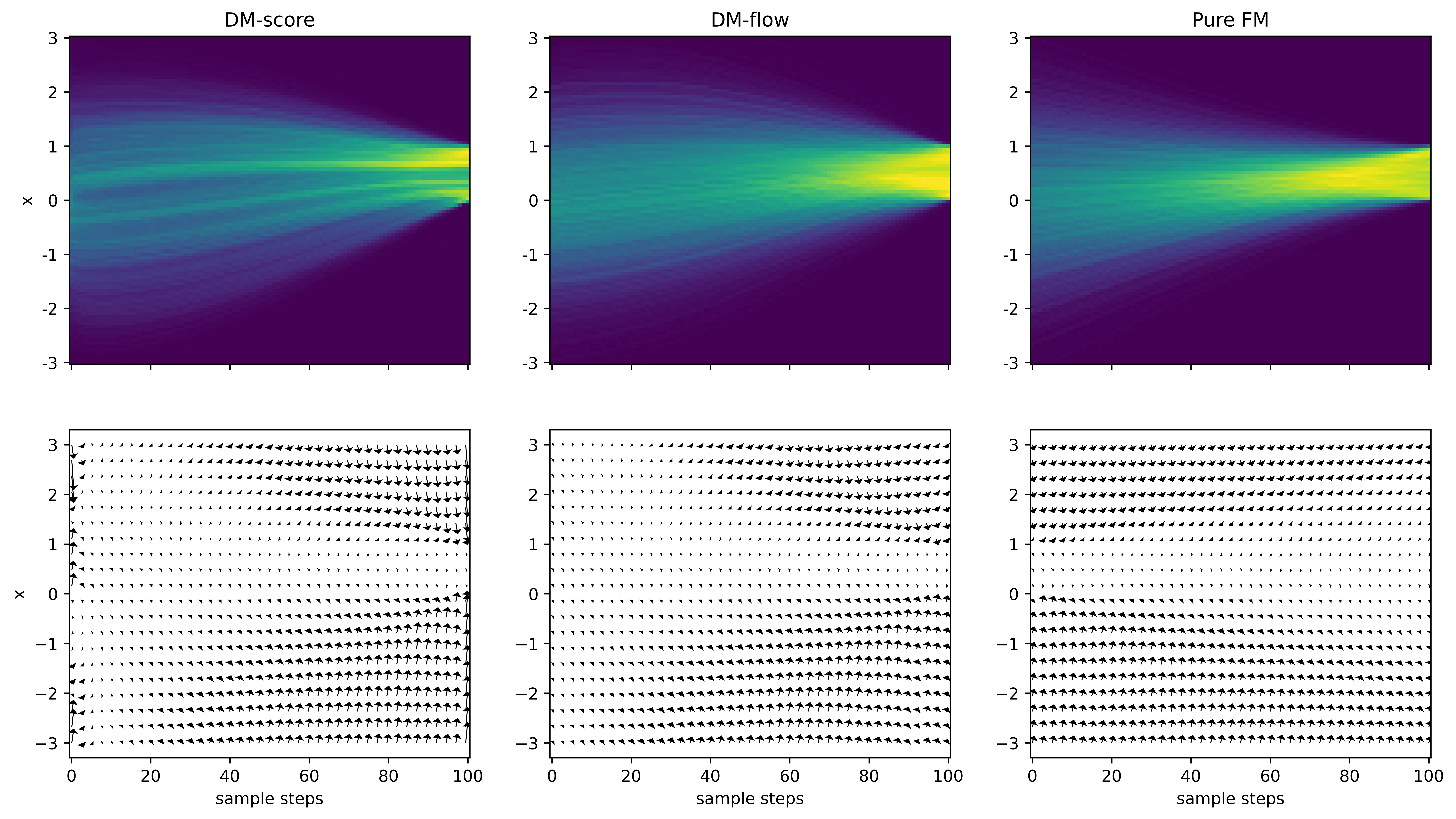
Straighter velocity fields means fewer steps for sampling generation. Compare -

• DM with score matching - non-smooth output even at 100 steps

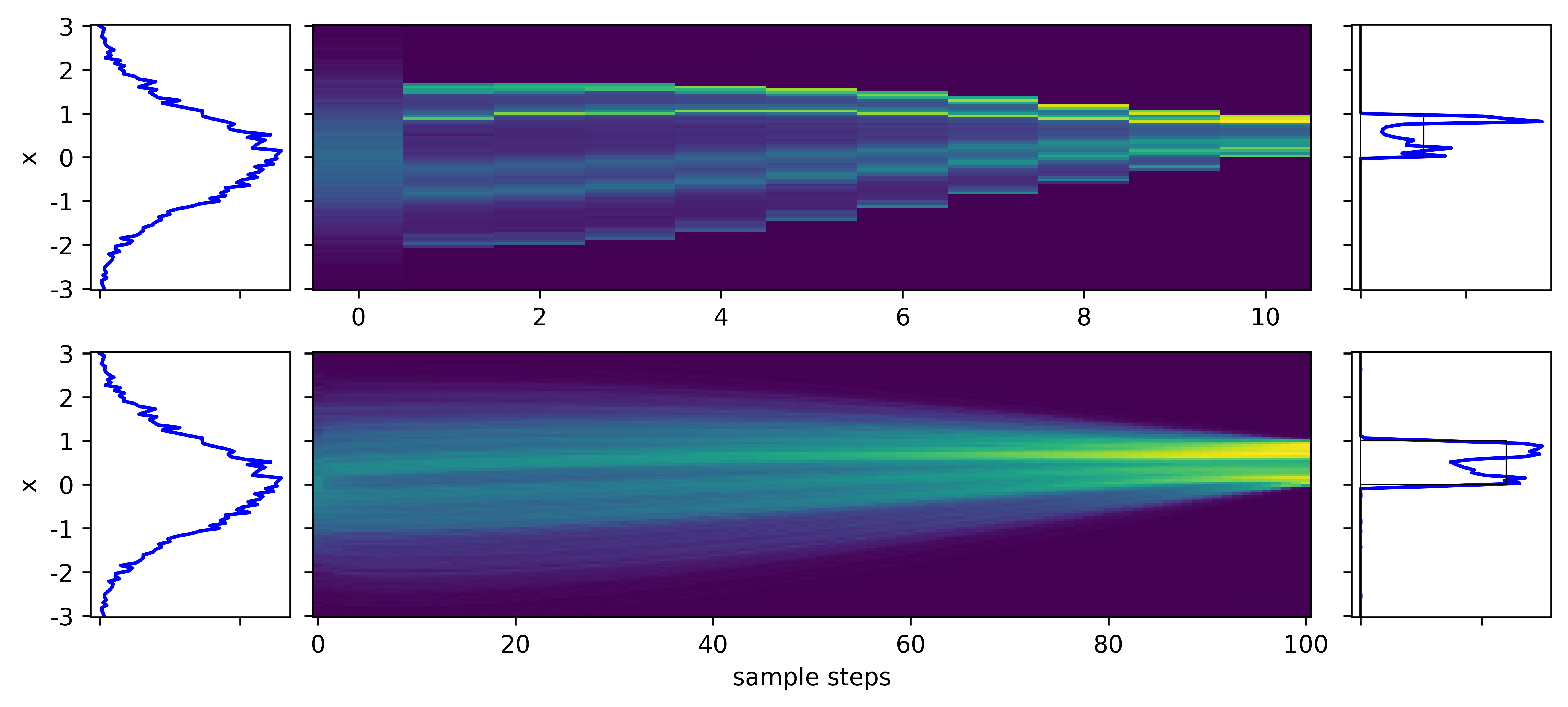
• DM with flow matching - already working at 10 steps

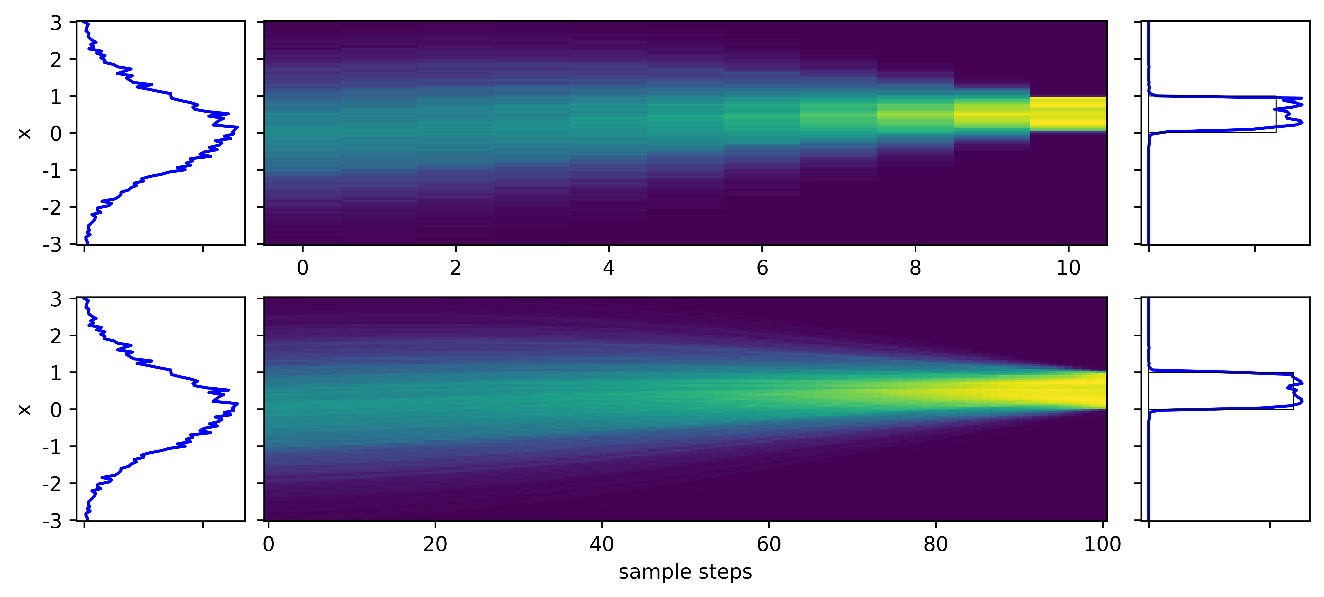
• Pure flow matching - also working at 10 steps, (and simpler formulation!)

Conditioned case

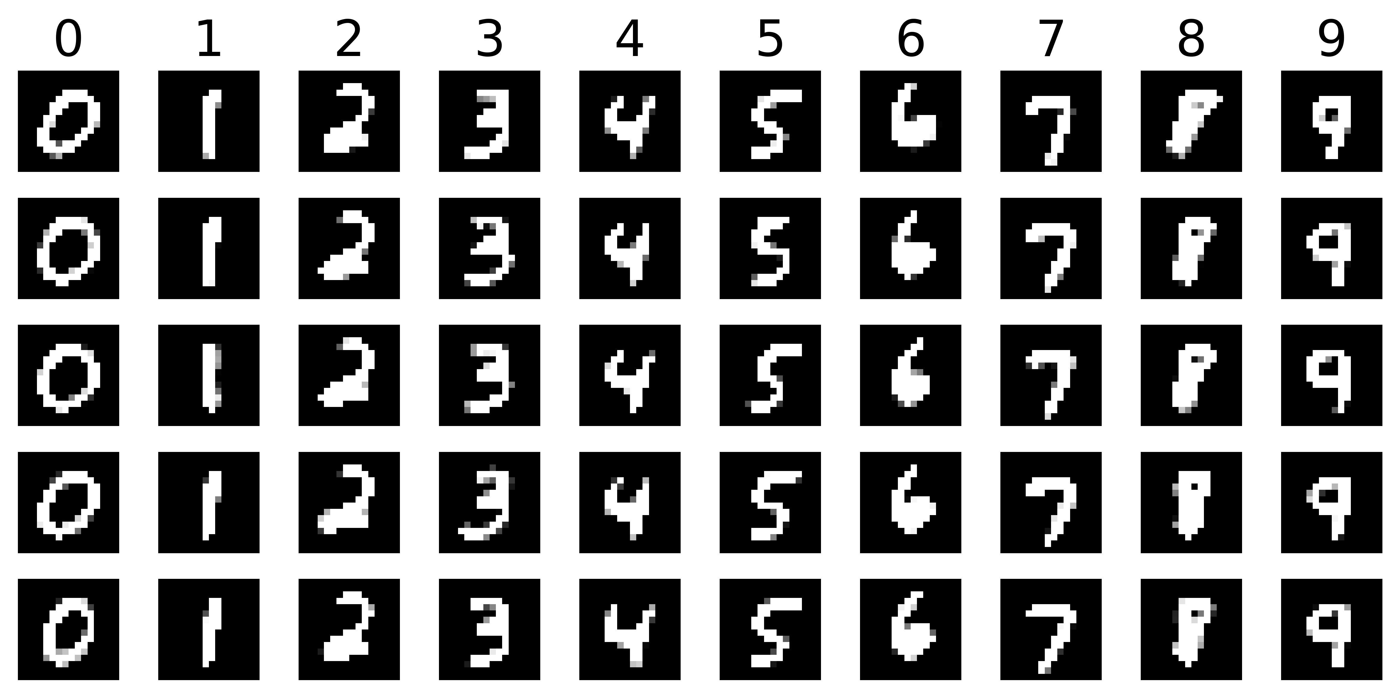
With better computational efficiency of FM, we can show an image example, instead of a 1D problem.

• The goal is to generate hand-written digits given the labels (0, 1, 2, ..., 9)
• Use a simple FiLM-like structure, so the label directly controls the velocity field

Some random samples for digits 0-9

Animated generation of digits 0-9 (after this, we clamp the pixel values to 0-1 to produce the final sample)