In L23, we have presented three underpinning principles for data-driven modeling of dynamical systems. The last one is that
Global linearization: A finite-dimensional nonlinear system can be represented by an infinite-dimensional linear system
We have shown a special example where the linear system is actually finite-dimensional, $$ \left\{\begin{array} \ \dot x_1 = \mu x_1 \\ \dot x_2 = \lambda (x_2-x_1^2) \end{array}\right. \Rightarrow \left\{\begin{array} \ \dot y_1 = \mu y_1 \\ \dot y_2 = \lambda (y_2-y_3) \\ \dot y_3 = 2\mu y_3 \end{array}\right. $$ where $$ y_1=x_1,\quad y_2=x_2,\quad y_3=x_1^2 $$
Here is one more example of PDE - 1D viscous Burgers' equation (model problem for shock waves) $$ \frac{\partial u}{\partial t}+u\frac{\partial u}{\partial x} = \nu \frac{\partial^2 u}{\partial x^2},\quad u(x,0)=f(x) $$
From Wikipedia, Cole-Hopf Transformation
Choosing $$ u = -2\nu\frac{1}{\phi}\frac{\partial \phi}{\partial x} $$ one gets a linear PDE that can be solved easily $$ \frac{\partial \phi}{\partial t} = \nu\frac{\partial^2 \phi}{\partial x^2} $$ (given the correct boundary conditions)
However...
In general, the "global linearization" in finite dimensions does not always work.
For example, if we modify the first example as $$ \begin{align} \dot x_1 &= \mu x_1 \\ \dot x_2 &= \lambda \color{red}{(x_2^2-x_1)} \end{align} $$ Then the previous strategy will result in a cascading problem, i.e. infinite $y_i$'s will be needed to make the transformed system linear, $$ \begin{align} \dot y_1 &= \mu y_1 \\ \dot y_2 &= \lambda (y_3-y_1) \\ \dot y_3 &= 2 \lambda (y_4-y_5) \\ \dot y_4 &= \cdots \\ \vdots &= \cdots \end{align} $$ where $$ y_1=x_1,\quad y_2=x_2,\quad y_3=x_2^2,\quad y_4=x_2^3,\quad y_5=x_1x_2,\quad \cdots $$
Koopman Operator (Discrete time)
Now let's formalize the "global linearization" procedure. Let's first start with the discrete time case, $$ \begin{align} \mbox{System dynamics: }&\ \vx_{k+1}=\vf(\vx_k) \\ \mbox{Observation: }&\ \vg_k=\vg(\vx_k) \\ \mbox{Initial condition: }&\ \vg_0=\vg(\vx_0) \end{align} $$
Next, let's first just consider one scalar observation $g(\vx)$ -
A Koopman operator $\cK_t$ is infinite-dimensional, linear, and, $$ \cK_t g = g\circ\vf $$
In the notation above, $\cK_t$ is a "functional" that takes in a function ($g$) and returns another function. $\circ$ means function composition.
Essentially, $\cK_t$ does the following, observable linearizing: $$ \cK_t g(\vx_k) = g(\vf(\vx_k)) = g(\vx_{k+1}) $$
The first step is by definition of $\cK_t$ and the second step is due to system dynamics
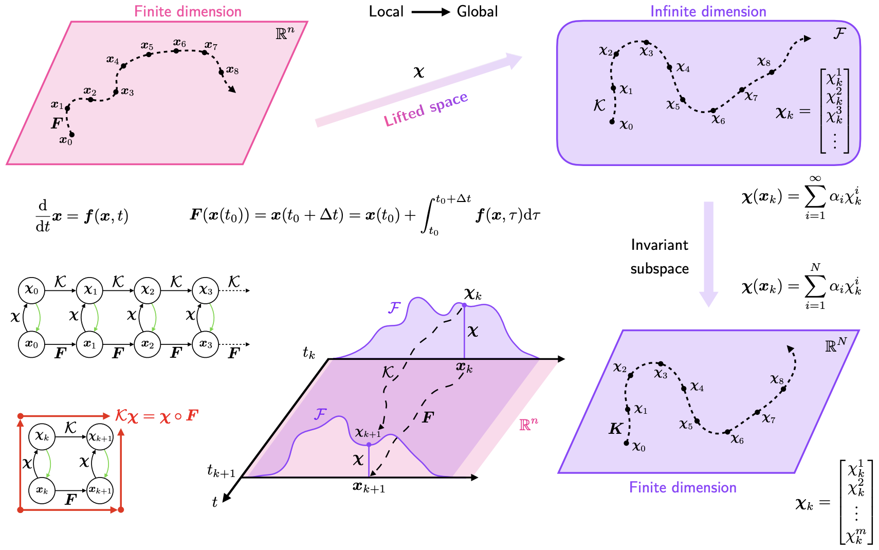
Figure Credit: Gueho, D., et al., DOI: 10.2514/6.2022-0655
$\cK_t$ is linear, so $$ \cK_t(c_1 g_1+c_2 g_2) = c_1 \cK_t g_1+c_2 \cK_t g_2 $$ for any scalars $c_1,c_2$ and any functions $g_1,g_2$.
And for linear transformations (even infinite dimensional), one can always define an eigenvalue problem $$ \cK_t\phi_i = \tilde{\lambda}_i\phi_i,\quad i=0,1,\cdots $$ where $\tilde{\lambda}_i$ are Koopman eigenvalues, and $\phi_i$ are Koopman eigenfunctions.
There are infinite number of eigenfunctions, since $\cK_t$ is infinite-dim
From a perspective of discrete-time system, one should expect $$ \tilde{\lambda}_i\phi_i(\vx_k) = \cK_t\phi_i(\vx_k) = \phi(\vf{\vx_k}) = \phi(\vx_{k+1}) $$
But the above "trivial" relation leads to an interesting lattice property - consider the product of two eigenfunctions $\phi(\vx)=\phi_i(\vx)\phi_j(\vx)$ $$ \begin{align} \cK_t(\phi(\vx)) &= \cK_t(\phi_i(\vx)\phi_j(\vx)) \\ &= \phi_i(\vf(\vx))\phi_j(\vf(\vx)) \\ &= \tilde{\lambda}_i\tilde{\lambda}_j\phi_i(\vx)\phi_j(\vx) \end{align} $$
The product of Koopman eigenfunctions is also a Koopman eigenfunction! Same for eigenvalues
Koopman Mode Decomposition
Just like eigenvectors in finite-dim space, eigenfunctions in infinite-dim space form a basis for representing other functions.
For a scalar observation function $g_i(\vx)$ $$ g_i(\vx) = \sum_{j=0}^\infty \xi_{ij}\phi_j(\vx) = \begin{bmatrix} \xi_{11} & \xi_{12} & \xi_{13} & \cdots \end{bmatrix} \begin{bmatrix} \phi_1(\vx) \\ \phi_2(\vx) \\ \phi_3(\vx) \\ \vdots \end{bmatrix} $$ where $\xi_{ij}$ are scalar coefficients.
When there are multiple observables, each observable can be expanded likewise, $$ \begin{bmatrix} g_1(\vx) \\ g_2(\vx) \\ \vdots \\ g_m(\vx) \end{bmatrix} = \begin{bmatrix} \xi_{11} & \xi_{12} & \xi_{13} & \cdots \\ \xi_{21} & \xi_{22} & \xi_{23} & \cdots \\ \vdots & \vdots & \vdots & \cdots \\ \xi_{m1} & \xi_{m2} & \xi_{m3} & \cdots \end{bmatrix} \begin{bmatrix} \phi_1(\vx) \\ \phi_2(\vx) \\ \phi_3(\vx) \\ \vdots \end{bmatrix} $$ Or in short, $$ \vg(\vx) = \sum_{i=0}^\infty \phi_i(\vx)\vtx_i $$ where $\vtx_i$ are columns of the coefficient matrix and called the Koopman modes.
This is the Koopman Mode Decomposition
Then, the time response is represented as $$ \vg(\vx_{k+1}) = \cK_t\vg(\vx_k) = \sum_{i=0}^\infty \cK_t\phi_i(\vx_k)\vtx_i = \sum_{i=0}^\infty \tilde{\lambda}_i\phi_i(\vx_k)\vtx_i $$
One can further go backwards in time $$ \begin{align} \vg(\vx_{k+1}) &= \cK_t^2\vg(\vx_{k-1}) = \sum_{i=0}^\infty \cK_t^2\phi_i(\vx_{k-1})\vtx_i = \sum_{i=0}^\infty \tilde{\lambda}_i^2\phi_i(\vx_{k-1})\vtx_i \\ &= \vdots \\ &= \sum_{i=0}^\infty \tilde{\lambda}_i^{k+1}\phi_i(\vx_0)\vtx_i \end{align} $$ where the initial condition is expanded as $$ \vg(\vx_0) = \sum_{i=0}^\infty \phi_i(\vx_0)\vtx_i $$
Looking familiar?
Recall
If we collect the observables as a time sequence, and apply DMD to identify a discrete linear system, $$ \vg_{k+1} = \vA \vg_k $$ where $\vA\in\bR^{m\times m}$ has eigenvalues $\lambda_i$ and eigenvectors $\vtf_i$ (i.e. the DMD modes).
Then the solution can be written as, $$ \vg_{k+1}=\sum_{i=1}^m b_i \lambda_i^{k+1} \vtf_i $$ where the initial condition is expanded as $$ \vg_0 = \sum_{i=1}^m b_i \vtf_i $$
It is clear there is a one-to-one correspondence
- DMD modes $\vtf_i$ v.s Koopman modes $\vtx_i$
- DMD eigenvalues $\lambda_i$ v.s. Koopman eigenvalues $\tilde{\lambda}_i$
- DMD modal coordinates $b_i$ v.s. Koopman eigenfunctions $\phi_i(\vx_0)$ (or more generally for any $\vx_k$)
Therefore DMD is an approximation of the Koopman operator via truncation.
This explains why DMD works for many nonlinear problems (having a low-dim linear structure, such as a limit cycle).
Extended DMD
The connection between DMD and Koopman also provides a means for numerical implementation of Koopman mode decomposition.
First, construct the data matrices as $$ \vG=[\vg_0,\vg_1,\cdots,\vg_N],\quad \vG^1=[\vg_1,\vg_2,\cdots,\vg_{N+1}] $$
From standard DMD, we can find the system matrix, together with its eigendecomposition, $$ \vA = \vG^1\vG^+ \approx \vtF\vtL\vtY^H $$ where $+$ is pseudo-inverse.
Based on previous discussion, $\vtL$ are simultaneously the DMD and Koopman eigenvalues
Next, let's recover the Koopman eigenfunctions.
An eigenfunction and its eigenvalue should satisfy $$ \begin{bmatrix} \lambda\phi(\vx_0) \\ \lambda\phi(\vx_1) \\ \vdots \\ \lambda\phi(\vx_N) \end{bmatrix} =\begin{bmatrix} \phi(\vx_1) \\ \phi(\vx_2) \\ \vdots \\ \phi(\vx_{N+1}) \end{bmatrix} $$
Think the observables as basis functions that approximate an eigenfunction, $$ \phi(\vx) \approx \sum_{i=1}^m g_i(\vx)u_i = \vg(\vx)^T\vu $$ Then $$ \begin{bmatrix} \phi(\vx_1) \\ \phi(\vx_2) \\ \vdots \\ \phi(\vx_{N+1}) \end{bmatrix} = \begin{bmatrix} \vg(\vx_1)^T \\ \vg(\vx_2)^T \\ \vdots \\ \vg(\vx_{N+1})^T \end{bmatrix}\vu = (\vG^1)^T\vu $$ and doing the same for the left-hand side $$ \lambda\vG^T\vu = (\vG^1)^T\vu $$
Thinking again in least squares, we get an eigenvalue problem $$ \lambda\vu = (\vG^T)^+(\vG^1)^T\vu = \vA^T\vu $$ So $\vu$ are the left eigenvectors of $\vA$, i.e. $\vtY$. In other words, EDMD approximates the Koopman eigenfunctions as $\vg(\vx)^T\vtY$.
Side note
Why can we truncate "safely" an infinite-dimensional system? There are several arguments
- From functional analysis, if one approximates a function by, say eigenfunctions $\{\phi_i\}_{i=1}^\infty$, the coefficients always decay as $i\rightarrow\infty$.
- From dynamical systems, the trajectory is more likely residing on a bounded low-dimensional structure (limit cycle, strange attractor, etc.), so a handful eigenfunctions might be sufficient to characterize the structure.
- The lattice property of $\cK_t$ indicates that, in at least some cases, the infinite eigenpairs might be simply generated by a finite set of eigenpairs.
Koopman Operator (Continuous time)
Now consider a dynamical system that is sufficiently smooth, $$ \begin{align} \mbox{System dynamics: }&\ \dot{\vx}=\vf(\vx) \\ \mbox{Observation: }&\ \vg=\vg(\vx) \\ \mbox{Initial condition: }&\ \vx(0)=\vx_0 \end{align} $$
One can seek the Koopman generator $$ \dot{g}=\cK g $$ where note that we drop the subscript $t$.
$\cK$ is essentially the infinitesimal limit of the Koopman operator, so that $$ \cK g = \lim_{t\rightarrow 0} \frac{\cK_t g-g}{t} = \lim_{t\rightarrow 0} \frac{g\circ\vf-g}{t} $$
In some sense, $\cK$ and $\cK_t$ are analogous to $\vA$ and $\exp(\vA t)$ for finite-dim linear systems.
Again $\cK$ is linear and we can define the eigensystem as $$ \cK\phi = \mu\phi $$ and by definition of $\cK$, $\mu\phi=\dot\phi$.
Similar to the discrete case, the eigensystem also has a lattice property, for $\phi=\phi_i\phi_j$ $$ \cK\phi = \dot\phi = \dot{\phi}_i\phi_j + \phi_i\dot{\phi}_j = \mu_i\phi_i\phi_j + \mu_j\phi_i\phi_j = (\mu_i + \mu_j)\phi_i\phi_j $$
In fact, $\lambda=\exp(\mu\Delta t)$, which explains the difference in the lattices of $\cK_t$ (multiplicative) and $\cK$ (additive)
Taking a further look at $\dot{\phi}$, by chain rule, $$ \dot\phi(\vx) = \nabla\phi(\vx)\cdot\dot{\vx} = \nabla\phi(\vx)\cdot\vf(\vx) $$ where $\nabla$ is gradient w.r.t. $\vx$.
This leads to an alternative eigenvalue problem in the form of PDE $$ \mu\phi(\vx) = \nabla\phi(\vx)\cdot\vf(\vx) $$
This provides another approach to computing $\phi$ if $\vf$ is known
EDMD, Cont'd
If $\vf$ is unknown, which is most of the case, one could develop a continuous version of EDMD starting from the eigenvalue problem $$ \mu\phi(\vx) = \nabla\phi(\vx)\cdot\dot{\vx} $$
If one introduce the approximation $$ \phi(\vx) \approx \sum_{i=1}^m g_i(\vx)u_i = \vg(\vx)^T\vu $$ The eigenvalue problem becomes $$ \begin{align} \mu\left(\sum_{i=1}^m g_i(\vx)u_i\right) &= \nabla\left( \sum_{i=1}^m g_i(\vx)u_i \right)\cdot\dot{\vx} \\ \mu\vg(\vx)^T\vu &= \sum_{i=1}^m \left( \nabla g_i(\vx)\cdot \dot{\vx}\right) u_i \end{align} $$
From a series of data, $$ \mu\begin{bmatrix}\vg(\vx_1)^T \\ \vg(\vx_2)^T \\ \cdots \\ \vg(\vx_N)^T\end{bmatrix}\vu = \begin{bmatrix} \nabla g_1(\vx)\cdot \dot{\vx}_1 & \nabla g_2(\vx)\cdot \dot{\vx}_1 & \cdots & \nabla g_m(\vx)\cdot \dot{\vx}_1 \\ \nabla g_1(\vx)\cdot \dot{\vx}_2 & \nabla g_2(\vx)\cdot \dot{\vx}_2 & \cdots & \nabla g_m(\vx)\cdot \dot{\vx}_2 \\ \vdots & \vdots & \ddots & \vdots \\ \nabla g_1(\vx)\cdot \dot{\vx}_N & \nabla g_2(\vx)\cdot \dot{\vx}_N & \cdots & \nabla g_m(\vx)\cdot \dot{\vx}_N \end{bmatrix}\vu $$ Or in short $$ \mu\vG\vu = \vtG\vu $$
Yet another eigenvalue problem!
But since $\dot{\vx}$ is involved, a natural idea is to use SINDy, which also helps selecting the observables (i.e. features). See [1] for more details.
[1] Kaiser, E., et al., Data-driven discovery of Koopman eigenfunctions for control, 2021.
A touch on Control
Finally let's look at a nonlinear system with control, $$ \begin{align} \mbox{System dynamics: }&\ \dot{\vx}=\vf(\vx,\vu) \\ \mbox{Observation: }&\ \vg=\vg(\vx,\vu) \end{align} $$
This topic is still in active research and there are still some fundamental challenges.
In general, for a scalar observable, one can find $$ \dot{g} = \cK^\vu g $$ where $\cK^\vu$ is a linear non-autonomous Koopman operator, that depends on the control input $\vu$.
Like before, let's consider the eigenfunctions $$ \dot\phi = \cK^\vu \phi = \mu^\vu \phi $$
If we factor in the actual dynamics $\vf(\vx,\vu)$ $$ \mu^\vu \phi = \cK^\vu \phi = \dot{\phi} = \nabla_\vx \phi \cdot \vf(\vx,\vu) + \nabla_\vu \phi \cdot \dot{\vu} $$
Problem: What is $\dot\vu$?
This produces non-causal system that is inconvenient to analysis, even in classical control methods.
- So we set $\dot\vu=0$ and assume step changes in control inputs (i.e. zero-hold)
One gets $$ \dot{\phi} = \nabla_\vx \phi \cdot \vf(\vx,\vu) $$
Problem: $\vf(\vx,\vu)$ is too generic, can we try something more tangible?
- So to make life even easier, we assume a control-affine system, $$ \dot{\vx} = \vf_0(\vx) + \sum_{i=1}^L \vf_i(\vx)u_i $$ where the system is linear in $\vu$.
- The autonomous part $\vf^0$ has a Koopman form $$ \mu^\vf\phi = \cK^\vf \phi = \dot{\phi} = \nabla_\vx \phi \cdot \vf_0(\vx) $$
The eigenproblem simplifies to $$ \begin{align} \dot\phi &= \nabla_\vx \phi \cdot \vf_0(\vx) + \sum_{i=1}^L \nabla_\vx \phi \cdot \vf_i(\vx)u_i \\ &= \mu^\vf \phi + \sum_{i=1}^L \nabla_\vx \phi \cdot \vf_i(\vx)u_i \end{align} $$
Problem: What about the second part?
- Let's assume $\nabla_\vx \phi \cdot \vf_i(\vx)$ can be approximated by a specific set of eigenfunctions $\{\phi_j\}_{j=1}^P$ $$ \nabla_\vx \phi \cdot \vf_i(\vx) = \sum_{j=1}^P b_{ij}\phi_j $$
Then for the $k$th eigenfunction, $$ \dot{\phi}_k = \mu_k^\vf\phi_k + \sum_{i=1}^L \sum_{j=1}^P b_{ij}^k\phi_j u_i \equiv \mu_k^\vf\phi_k + (\vB^k\vtf)^T \vu $$ And if one write the equation for the $P$ eigenfunctions, $$ \dot\vtf = \vtL\vtf + \begin{bmatrix} \vB^1\vtf & \vB^2\vtf & \cdots & \vB^P\vtf \end{bmatrix}^T\vu = \vtL\vtf + (\cB\vtf) \vu $$
- $\vtL$ is a diagonal matrix with eigenvalues $\{\mu_j\}_{j=1}^P$
- $\cB$ is a "3D matrix", or a so-called bilinear operator
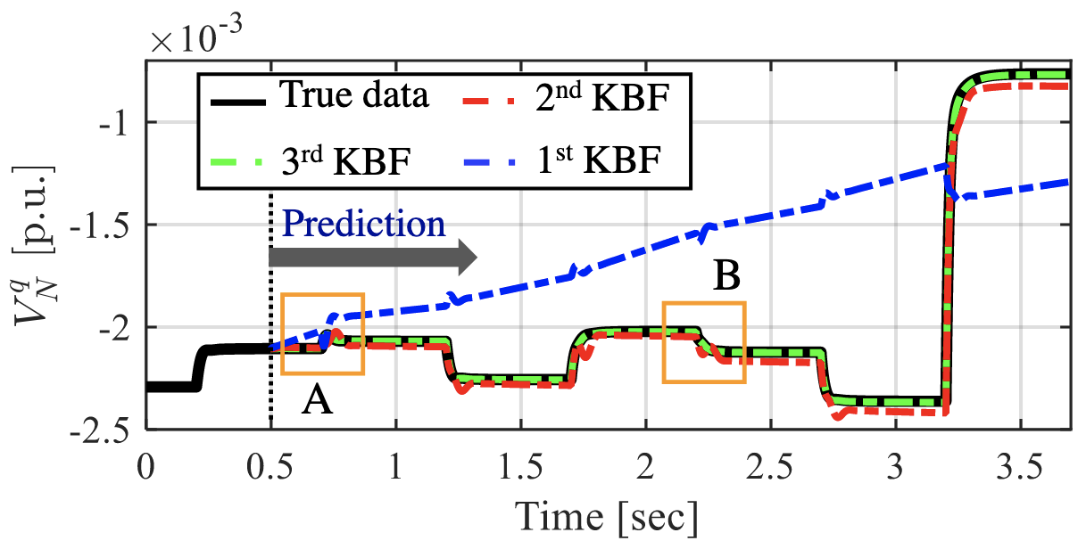
Now we get a working Koopman Bilinear Form
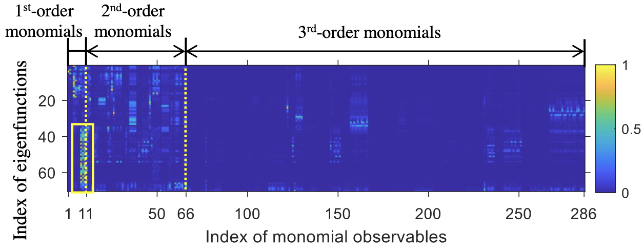
- We can apply a modified EDMD technique to find the coefficients and the eigenfunctions, see [Brunton2022]
Two examples
Example 1
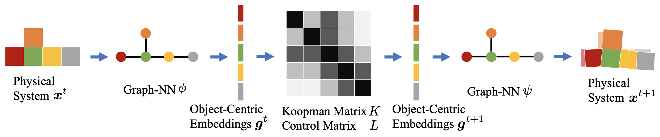
Ref: Li, Y., et al., Learning compositional Koopman operators for model-based control, 2019.
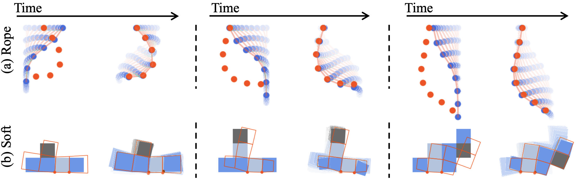
Ref: Li, Y., et al., Learning compositional Koopman operators for model-based control, 2019.
In-house work