TODAY: Dynamical System
- Recap
- Underpinning principles
- Low-dimensional representation
- Time delay embedding
- Infinite-dimensional linear representation
Recap
Where we are now
So far we have dealt mainly with linear systems.
In terms of notations above, we now know how to find $$ y_{k+1} = A y_k $$ given high-dimensional observations $\{y_k\}_{k=1}^N$.
- Also how to extract useful information from it (stability, input/output modes, etc.)
Certainly this is not sufficient, we at least want to know $$ \begin{align} x_{k+1} &= Ax_k + Bu_k \\ y_k &= Cx_k + Du_k \end{align} $$ For this we have many algorithms for example,
- Eigensystem realization algorithm (ERA) [1] plus Observer/Kalman Identification Algorithm (OKID) [2]
- The subspace methods (e.g.
n4sidin MATLAB - see its documentation) - Balanced truncation/Balanced POD [3]
[1] Juang, J.-N., et al., An Eigensystem Realization Algorithm for Modal Parameter Identification and Model Reduction, 1985.
[2] Juang, J.-N., et al., Identification of Observer/Kalman Filter Markov Parameters: Theory and Experiments, 1993.
[3] Rowley, C., Model Reduction for Fluids, Using Balanced Proper Orthogonal Decomposition, 2005.
In fact, we can also handle linear systems that are time-varying and parametric $$ \begin{align} x_{k+1} &= A(t_k,\mu)x_k + B(t_k,\mu)u_k \\ y_k &= C(t_k,\mu)x_k + D(t_k,\mu)u_k \end{align} $$ There are also algorithms for these, for example, Time-varying ERA [1]
Unfortunately we don't have time to cover all the above methods in detail.
[1] Majji, M., et al., Time-Varying Eigensystem Realization Algorithm, 2010.
The initially posed question was ...
For a nonlinear system:
$$ \begin{align} \dot{x} &= f(x,t,u;\mu) + d,\quad x(0)=x_0 \\ y_k &= g(x_k,t_k,u_k;\mu) + \epsilon \end{align} $$Given
- Trajectories $D=\{(t_i,u_i,\mu_i,y_i)\}_{i=1}^N$
- Possibly also knowledge about the problem
- Physical properties: conservativeness, stability, etc.
- Part of governing equations
Identify $$ \begin{align} \dot{x} &= \hat{f}(x,t,u;\mu),\quad x(0)=x_0 \\ y_k &= \hat{g}(x_k,t_k,u_k;\mu) \end{align} $$
- To reproduce the given data and generalize to unseen data
- If possible provide an error estimate on the prediction
How do we go about it?
Three underpinning principles
Low-dimensional representation
As we have seen in the previous module:
High-dimensional data typically lives in a low-dimensional space
If we represent the high-dimensional data $x\in\bR^{N}$ as $$ x = \Phi \xr{} + \Phi^\perp \xt{} $$ where $\Phi\in\bR^{N\times N_r}$ and $\Phi^\perp\in\bR^{N\times N_t}$, $N=N_r+N_t$, and $N\gg N_r$.
We call $\Phi$ the trial basis, due to a connection to finite element method.
The basis $\Phi$ and $\Phi^\perp$ are mutually orthogonal.
- So any two vectors $\Phi \xr{}$ and $\Phi^\perp \xt{}$ are orthogonal to each other.
- In high-dimension, we shall expect that, with a properly chosen $\Phi$ $$ x\approx \Phi\xr{}\equiv \tilde{x} \quad\mbox{or}\quad \frac{\norm{x-\Phi \xr{}}}{\norm{x}} \ll 1 $$ where $\xr{}=\Phi^+ x=(\Phi^T\Phi)^{-1}\Phi^T x$
Linear case
Consider a high-dimensional linear system, $A\in\bR^{N\times N}$ $$ \begin{align} x_{k+1} &= Ax_k + Bu_k \\ y_k &= Cx_k + Du_k \end{align} $$ and approximate the solution using the trial basis $$ \begin{align} \Phi\xr{k+1} &= A\Phi \xr{k} + B u_k \\ y_k &= C\Phi \xr{k} + Du_k \end{align} $$
Further, introduce a test basis $\Psi\in\bR^{N\times N_r}$, and left-multiply $\Psi^T$ $$ \begin{align} \xr{k+1} &= (\Psi^T\Phi)^{-1}\Psi^TA\Phi \xr{k} + (\Psi^T\Phi)^{-1}(\Psi^TB) u_k \\ y_k &= (C\Phi) \xr{k} + Du_k \end{align} $$ where the system matrice is much smaller $$ A_r\equiv(\Psi^T\Phi)^{-1}\Psi^TA\Phi \in \bR^{N_r\times N_r} $$
Computational cost reduces from $O(N^2)$ to $O(N_r^2)$
Nonlinear case
Next, we turn to a nonlinear model but without inputs or outputs, for simplicity $$ \dot{x} = f(x),\quad x(0)=x_0 $$
Again using a trial basis $\Phi$, one finds $$ \Phi\dot{\xr{}} = f(\Phi\xr{}),\quad \Phi\xr{}(0)=x_0 $$
Using a test basis $\Psi$, and assuming that $(\Psi^T\Phi)$ is non-singular, $$ \dot{\xr{}} = (\Psi^T\Phi)^{-1}\Psi^T f(\Phi\xr{}),\quad \xr{}(0)= (\Psi^T\Phi)^{-1}\Psi^T x_0 $$ Recovering the full-order system $$ \dot{\tilde{x}} = \Pi_{\Phi,\Psi} f(\tilde{x}),\quad \tilde{x}(0)= \Pi_{\Phi,\Psi} x_0 $$ where $\tilde{x}=\Phi\xr{}$ we have defined a Petrov-Galerkin projection operator $$ \Pi_{\Phi,\Psi}=\Phi(\Psi^T\Phi)^{-1}\Psi^T $$
Error analysis
Next consider the error due to projection. To make things easier to "imagine",
- Assume that $\Phi$ is orthonormal, so that $\Phi^T\Phi=I$.
- Let the trial basis $\Psi=\Phi$ - this is called Galerkin projection.
- The projection operator becomes more familiar (hopefully) $\Pi=\Phi\Phi^T$.
The error is decomposed as $$ \begin{align} \epsilon &= x-\tilde{x} \\ &= x - \Pi x + \Pi x - \Phi \xr{} \\ &= (I-\Pi)x + \Phi(\Phi^T x - \xr{}) \\ &= \epsilon_\perp + \epsilon_\parallel \end{align} $$
- $\epsilon_\perp$ is "out of plane" and we cannot control
- $\epsilon_\parallel$ is "in plane" and possibly controllable
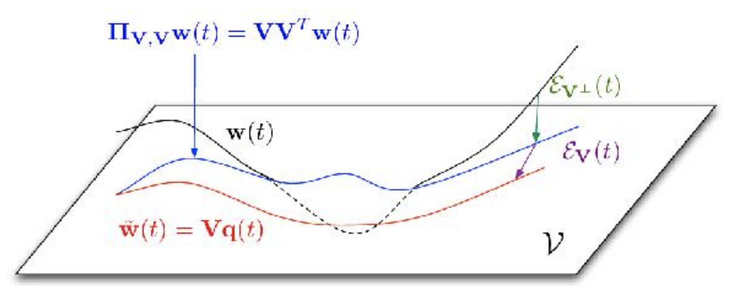
Figure from Stanford CME345 Ch3, by C. Farhat.
For the in-plane error, $$ \begin{align} \dot{\epsilon}_\parallel &= \frac{d}{dt}\left[ \Phi(\Phi^T x - \xr{}) \right] \\ &= \Phi\Phi^T \dot{x} - \dot{\tilde{x}} \\ &= \Pi f(x) - \Pi f(\tilde{x}) \\ &= \Pi \left[ f(x) - f(x-\epsilon_\perp-\epsilon_\parallel) \right] \end{align} $$ The in-plane error is impacted by the out-of-plane error that is not controllable!
At least in this vanilla projection-based formulation
Further development
The key ideas behind the projection-based ROM is essentially
- Projection: Map from the high-dim state space to a low-dim latent space
- Update: Compute the state evolution in latent space
- Reconstruction: Map the updated latent state to the original space
In the classical approach,
- Projection and Reconstruction are done by linear bases
- Update requires not only the availability of the simulation code but also an intrusive modification of the code.
From a data-driven perspective,
- Projection and Reconstruction can be done by autoencoders
- More accurate reconstruction
- Adaptable to different parameters $$ \xr{} = \Phi(x,\mu),\quad x=\Psi(\xr{},\mu) $$
- Update can be done by any data-driven time series models, e.g., vanilla NN, LSTM, etc.
- Bypasses the need for the simulation code
- Could mix with part of the code (e.g. the linear part) if necessary $$ \xr{k+1} = F(\xr{k}) $$
Possible complaints - now we got a purely black-box model that we don't know how it works!
Side note
- One way to mitigate the impact of out-of-plane error is through Residual Minimization. See [1] for more details.
- For a dynamical system with parameter $\mu$, one can first construct a set of bases $\{\Phi(\mu_i)\}_{i=1}^K$, find the basis at a new parameter $\mu^*$ by, e.g. Grassmannian interpolation, and then find the new ROM using $\Phi(\mu^*)$. See [2] for more details.
- Unlike the linear case, the computational cost for nonlinear problem reduces from $O(N^2)$ to $O(N N_r)$, due to the need for evaluating the $N$-dimensional $f$ function. There are ways to reduce this cost as well. See [3] for more details.
[1] Carlberg, K., et al., Galerkin v. least-squares Petrov-Galerkin projection in nonlinear model reduction, 2016.
[2] Amsallem, D., et al., Nonlinear model order reduction based on local reduced‐order bases, 2012.
[3] Carlberg, K., et al., The GNAT method for nonlinear model reduction, 2013.
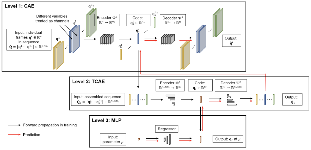
Example: Ship airwake with sideslip angle
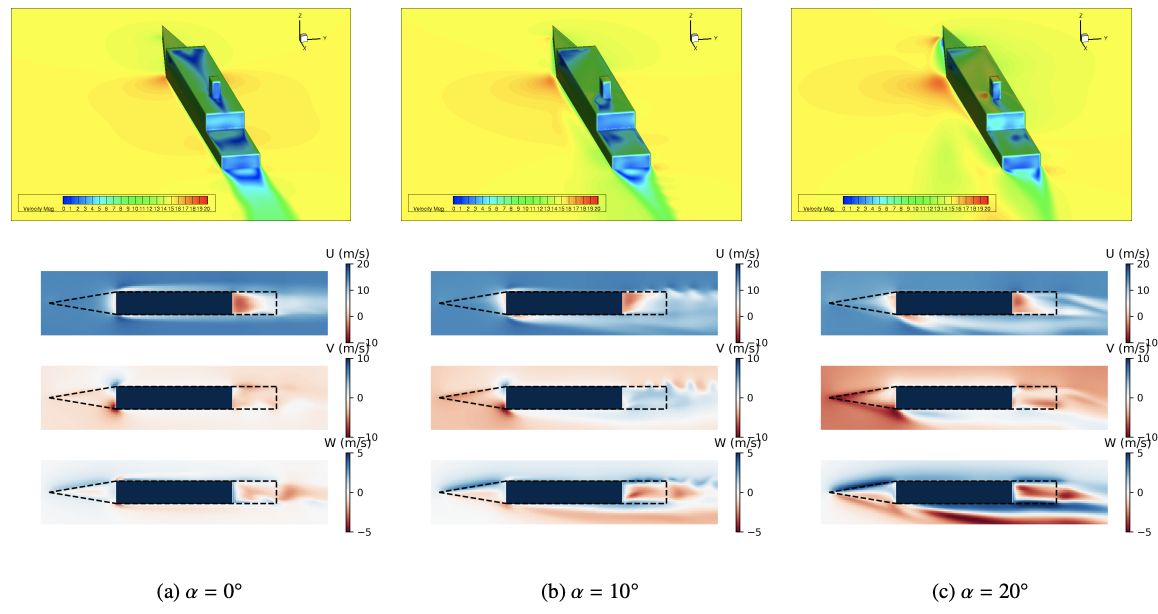
[1] Xu, J., et al., Multi-level Convolutional Autoencoder Networks for Parametric Prediction of Spatio-temporal Dynamics, 2020.
[1] Xu, J., et al., Multi-level Convolutional Autoencoder Networks for Parametric Prediction of Spatio-temporal Dynamics, 2020.
Time delay embedding
In 1981 Floris Takens developed a delay embedding theorem for chaotic dynamical systems. The essential implication is
Unobservable information of a dynamical system is recovered from the time history of the observables.
Starting with the linear system without output, for simplicity.
Suppose we plan to retain some states $\xr{}$ (e.g. by linear projection) and truncate the rest $\xt{}$.
Formally we can write, $$ \begin{align} \begin{bmatrix} \xr{k+1} \\ \xt{k+1} \end{bmatrix} &= \begin{bmatrix} A^{rr} & A^{rt} \\ A^{tr} & A^{tt} \end{bmatrix} \begin{bmatrix} \xr{k} \\ \xt{k} \end{bmatrix} + \begin{bmatrix} B^{r} \\ B^{t} \end{bmatrix}\color{blue}{u_k} \end{align} $$
The reduced states are governed by $$ \color{blue}{x_{k+1}^r} = A^{rr}\color{blue}{x_k^r} + A^{rt}\color{red}{x_k^t} + B^r\color{blue}{u_k} $$ which is impacted by the truncated states, as we have seen in the previous section.
But the other equation can help to substitute the unknown states $$ \color{red}{x_k^t} = A^{tr}\color{blue}{x_{k-1}^r} + A^{tt}\color{red}{x_{k-1}^t} + B^t\color{blue}{u_{k-1}} $$ $$ \color{red}{x_{k-1}^t} = A^{tr}\color{blue}{x_{k-2}^r} + A^{tt}\color{red}{x_{k-2}^t} + B^t\color{blue}{u_{k-2}} $$
Though we got new unknown states...
But if we continue to do the substitution, $$ \begin{align} \color{blue}{x_{k+1}^r} &= A^{rr}\color{blue}{x_k^r} + \sum_{i=1}^{K} A^{rt}(A^{tt})^{i-1}A^{tr}\color{blue}{x_{k-i}^r} \\ &+ A^{rt}(A^{tt})^K \color{red}{x_{k-K-1}^t} \\ &+ B^r\color{blue}{u_k} + \sum_{i=1}^{K} A^{rt}(A^{tt})^{i-1}B^t\color{blue}{u_{k-i}} \end{align} $$
- $\color{blue}{x_{k-i}^r}$: Past known states
- $\color{red}{x_{k-K-1}^t}$: The only unknown state
- $\color{blue}{u_{k-i}}$: Past known inputs
If $(A^{tt})^K$ is sufficiently small, then the unknown state has negligible impact on the dynamics; Or, the system "forgets" the past state
Generalizing for the nonlinear problem, we obtain the classical Nonlinear AutoRegressive eXogenous model (NARX) $$ x_{k+1}^r = F(\{x_{k-i}^r\}_{i=0}^K,\{u_{k-i}\}_{i=0}^K) + \epsilon $$ where $\epsilon$ consists of approximation error and data noise.
Furthermore, Takens' theorem says that the approximation is exact when $K$ is sufficiently large
Some people also call this Mori-Zwanzig formalism due to a connection to the statistical physics.
# A literal "embedding" example
# Left: Seemingly irregular dynamics (different init. conds.)
# Right: Clear parabolic patterns using time delay coordinates
timeDelay([0.3, 0.4, 0.7], 4.0)

In some sense the above results indicate the underpinning principle for recurrent-type models, including
- Simple polynomial fits
- Recurrent NN, esp. LSTM
- Recurrent GPR
- etc.
All one needs is a nonlinear model for $F$, so that $$ x_{k+1}^r = F(\{x_{k-i}^r\}_{i=0}^K,\{u_{k-i}\}_{i=0}^K) $$
But in many cases a linear recurrent model is sufficient, even for nonlinear systems
Infinite-dimensional linear representation
AKA, Koopman theory
Low-dimensional nonlinear system is equivalent to an infinite-dimensional linear system.
We will spend a whole lecture on this topic. Here let's look at a classical example.
A 2D nonlinear system, $$ \begin{align} \dot x_1 &= \mu x_1 \\ \dot x_2 &= \lambda (x_2-x_1^2) \end{align} $$
Using the following coordinate transformation, $$ y_1=x_1,\quad y_2=x_2,\quad y_3=x_1^2 $$
We get a linear system, $$ \begin{align} \dot y_1 &= \mu y_1 \\ \dot y_2 &= \lambda (y_2-y_3) \\ \dot y_3 &= 2\mu y_3 \end{align} $$
In other words, for a nonlinear problem $$ \begin{align} \dot{x} &= f(x),\quad x(0)=x_0 \\ y_k &= g(x_k) \end{align} $$ One can find a nonlinear mapping $z_k=\varphi(y_k)$, so that $$ z_{k+1} = A z_k $$
We already know how to find $A$ if $z_k$ is given; the question is "just" to find the mapping $\varphi$
Next steps
As you might have noted, a common strategy for learning nonlinear dynamics is to reduce the high-dim state vector $x$ to a low-dim latent vector $\xr{}$, learn the latent dynamics $$ \dot{\xr{}} = F(\xr{}) $$ and transform back.
We have covered the dimensionality manipulation in the previous module.
So in the next few lectures we will present a few instances of algorithms for learning the latent dynamics.
- SINDy - A special version of linear regression
- NODE - Generalization of ResNet with roots in optimal control theory
- Koopman - A "reversed" approach that goes to infinite dimension