$$ \newcommand\norm[1]{{\left\lVert #1 \right\rVert}} \newcommand{\bR}{\mathbb{R}} \newcommand{\vf}{\mathbf{f}} \newcommand{\vg}{\mathbf{g}} \newcommand{\vv}{\mathbf{v}} \newcommand{\vw}{\mathbf{w}} \newcommand{\vx}{\mathbf{x}} \newcommand{\vy}{\mathbf{y}} \newcommand{\vA}{\mathbf{A}} \newcommand{\vB}{\mathbf{B}} \newcommand{\vU}{\mathbf{U}} \newcommand{\vV}{\mathbf{V}} \newcommand{\vW}{\mathbf{W}} \newcommand{\vX}{\mathbf{X}} \newcommand{\vtf}{\boldsymbol{\phi}} \newcommand{\vty}{\boldsymbol{\psi}} \newcommand{\vtF}{\boldsymbol{\Phi}} \newcommand{\vtS}{\boldsymbol{\Sigma}} \newcommand{\vtL}{\boldsymbol{\Lambda}} \newcommand{\cF}{\mathcal{F}} \newcommand{\cK}{\mathcal{K}} $$
TODAY: Dynamical System
- Simple linear regression
- The issues
- Sparse identification of nonlinear dynamics (SINDy)
- Sparsity-promotion
- Tackling noise
- Handling parameters
References
- [DMSC] Part 3
- [sindy2016] DOI: pnas.1517384113
- [PySINDy] DOI: 10.21105/joss.03994 and PySINDy@github
- See text for more references
Previously...
We have identified the basic problem to solve $$ \dot{x} = F(x) $$ where $x\in\bR^N$ consists of the full or partial state measurements, or reduced-order coordinates (e.g. after linear projection or autoencoder).
The nonlinear system function $F$ needs to be identified from $N$ trajectories $D=\{D_i\}_{i=1}^K$, where the $i$th trajectory of length $L_i$ is denoted $$ D_i=\left\{\left( t_j^{(i)},x_j^{(i)} \right)\right\}_{j=0}^{L_i} $$
Simple Linear Regression
Intuitively, we would like to have $$ \dot{x}_j^{(i)} = F(x_j^{(i)}) $$ for all data points.
If the time derivative is known, then this looks exactly like a linear regression problem.
Let's
- Assume $$ \begin{bmatrix} F_1(x) \\ F_2(x) \\ \vdots \\ F_N(x) \end{bmatrix} = \begin{bmatrix} \xi_{11} & \xi_{12} & \cdots & \xi_{1M} \\ \xi_{21} & \xi_{22} & \cdots & \xi_{2M} \\ \vdots & \vdots & \ddots & \vdots \\ \xi_{N1} & \xi_{N2} & \cdots & \xi_{NM} \end{bmatrix} \begin{bmatrix} \theta_1(x) \\ \theta_2(x) \\ \vdots \\ \theta_M(x) \end{bmatrix} \quad\mbox{or}\quad F(x)=\Xi^T\theta(x) $$ where $\Xi\in\bR^{M\times N}$ is the weight matrix to be fitted from data and $\theta(x) \in \bR^M$ is our familiar feature vector, such as polynomials $\theta_i(x)=x^{i-1}$.
- Approximate the time derivative by, e.g., finite difference, $$ \dot{x}_j^{(i)} \approx \frac{x_j^{(i)}-x_{j-1}^{(i)}}{t_j^{(i)}-t_{j-1}^{(i)}} $$
- For conciseness, consider just one trajectory - so we drop the $(i)$ in the following.
Then given all the sample trajectories, one can form a linear regression problem $$ \min_{\Xi} \norm{\dot X - \Theta(X)\Xi} $$ where $X$ and $\dot{X}$ contain the data row-wise, i.e., $$ X^T = [x_0,x_1,\cdots,x_{M}],\quad \dot{X}^T = [\dot{x}_0,\dot{x}_1,\cdots,\dot{x}_{M}] $$ and $$ \Theta(X)^T = [\theta(x_0),\theta(x_1),\cdots,\theta(x_{M})] $$
We should know very well by now how to solve the minimization problem, $$ \Xi = \Theta^+\dot{X} $$ where $\Theta^+$ is pseudo-inverse.
Let's see whether this formulation works
Model problem
A problem similar to what we encountered in resolvent analysis $$ \begin{bmatrix} \dot{x} \\ \dot{y} \end{bmatrix} = \begin{bmatrix} -\omega y - x r^2(r^2-\mu) \\ \omega x - y r^2(r^2-\mu)\end{bmatrix} $$ where $r^2=x^2+y^2$.
- When $\mu<0$, there is a stable equilibrium point at origin
- When $\mu\geq 0$, there is a stable limit cycle of radius $\sqrt{\mu}$, but an unstable equilibrium point at origin
OM, MU = 10, 4    # Picking omega=10, mu=4
func = lambda x: fSysNLn(0, x, om=OM, rr=MU)
pltQuiver([-3,3], 25, func, rr=2)

# Suppose now we generate the following two sample trajectories for training
dt = 0.0001    # Step size
Tf = 1.0       # Total time period
eps = 0.0      # Noise
x0s = [[1,0], [3,3]]  # Two initial conditions
t_train, x_train = genDataFixPar(dt, Tf, eps, x0s, (OM, MU))

# And we also generate two test trajectories
x0t = [[-0.5,-0.5], [-2,3]]  # Two initial conditions
t_test, x_test = genDataFixPar(dt, Tf, eps, x0t, (OM, MU))
# As expected, all trajectories converge to the limit cycle
# But the test trajectories cover a different region in state space.
cmpTrajPhase(x_train, x_test, ['Train', 'Test'])

Let's pick the following linear regression form $$ \begin{bmatrix} \dot{x} \\ \dot{y} \end{bmatrix} = \Xi^T\theta(x) = \begin{bmatrix} 0 & -\omega & \mu & 0 & -1 & 0 \\ \omega & 0 & 0 & \mu & 0 & -1 \end{bmatrix} \begin{bmatrix} x \\ y \\ xr^2 \\ yr^2 \\ xr^4 \\ yr^4 \end{bmatrix} $$
- $\Xi$ is what we need to find from data. The exact solution should be $$ \begin{bmatrix} 0 & -10 & 4 & 0 & -1 & 0 \\ 10 & 0 & 0 & 4 & 0 & -1 \end{bmatrix} $$
# Now we use the PySINDy implementation to do the fit
model = ps.SINDy(
    differentiation_method=ps.FiniteDifference(order=2),
    feature_library=clib_lco,             # We have pre-defined the feature vectors
    optimizer=ps.STLSQ(threshold=1e-4),   # This is almost like simple linear regression
    feature_names=["x", "y"])
model.fit(x_train, t=t_train, multiple_trajectories=True)
model.print()
print('\nFitted coefficients - not bad!')
model.coefficients()
(x)' = -0.007 x + -9.963 y + 4.011 xr^2 + -0.019 yr^2 + -1.002 xr^4 + 0.002 yr^4
(y)' = 9.994 x + 0.036 y + 0.011 xr^2 + 3.982 yr^2 + -0.002 xr^4 + -0.998 yr^4

Fitted coefficients - not bad!
array([[-0.0066, -9.9631,  4.0110, -0.0189, -1.0024,  0.0024],
       [ 9.9936,  0.0360,  0.0107,  3.9816, -0.0023, -0.9977]])
# The learned model performs very well on unseen data
x_pred = predTrajFixPar(model, x0t, t_train)
cmpTraj2D(x_test, x_pred, t_train, 2)
Solving [-0.5, -0.5]
Solving [-2, 3]

# Another comparison on the phase plane
cmpPhasePlane((OM,MU), [model], ['Learned'])

However ...
Here we have cheated to some degree
- We have chosen the features to be exactly those nonlinear terms in the exact model
- What if we do not know these features beforehand?
- If we just try as many features as we could think of, would the model overfit?
- We have delibrately used noise-free data with a tiny time step size
- With a larger time step size $\dot{X}$ would be less accurate
- Noise would make $\dot{X}$ even less accurate
- Perhaps we could try some filtering first on the data?
Next let's take a closer look at the feature selection and the denoising problem.
Feature selection: Sparse identification
If we do not know the model form beforehand, then it makes sense to try many many different features.
Back to the example
Say we only know that the model problem consists of polynomial terms, and we assume a feature vector of monomials up to 5th order, $$ \theta([x,y])^T = [x,y,x^2,xy,y^2,x^3,x^2y,xy^2,y^3,\cdots,xy^4,y^5] $$
The actual model, expanded in monomials, only consists of a tiny subset of the features, $$ \begin{bmatrix} \dot{x} \\ \dot{y} \end{bmatrix} = \begin{bmatrix} -\omega y - x r^2(r^2-\mu) \\ \omega x - y r^2(r^2-\mu)\end{bmatrix} = \begin{bmatrix} -\omega y + \mu x^3 + \mu xy^2 - x^5-2x^3y^2-xy^4 \\ \omega x + \mu x^2y + \mu y^3 - x^4y-2x^2y^3-y^5 \end{bmatrix} $$
But let's fit the model anyways.
model_overfit = ps.SINDy(
    differentiation_method=ps.FiniteDifference(order=2),
    feature_library=ps.PolynomialLibrary(degree=5),     # Now we use monomials up to 5th order
    # feature_library=ps.FourierLibrary(),
    optimizer=ps.STLSQ(threshold=1e-4),
    feature_names=["x", "y"])
model_overfit.fit(x_train, t=t_train, multiple_trajectories=True)
model_overfit.print()
print('\nFitted coefficients - cannot be true as they are all non-zero!')
(x)' = 6.983 1 + -6.383 x + -16.805 y + -2.350 x^2 + 7.366 x y + -1.197 y^2 + 5.719 x^3 + 1.852 x^2 y + 3.463 x y^2 + 2.317 y^3 + 0.151 x^4 + -1.841 x^3 y + 0.014 x^2 y^2 + -1.842 x y^3 + -0.137 y^4 + -1.031 x^5 + -0.038 x^4 y + -1.498 x^3 y^2 + -0.192 x^2 y^3 + -0.467 x y^4 + -0.154 y^5
(y)' = 6.807 1 + 3.779 x + -6.633 y + -2.291 x^2 + 7.180 x y + -1.167 y^2 + 1.675 x^3 + 5.805 x^2 y + -0.524 x y^2 + 6.259 y^3 + 0.147 x^4 + -1.795 x^3 y + 0.014 x^2 y^2 + -1.795 x y^3 + -0.133 y^4 + -0.030 x^5 + -1.037 x^4 y + 0.490 x^3 y^2 + -2.187 x^2 y^3 + 0.520 x y^4 + -1.150 y^5

Fitted coefficients - cannot be true as they are all non-zero!
# Prediction for train trajectories works well
x_pred = predTrajFixPar(model_overfit, x0s, t_train)
cmpTraj2D(x_train, x_pred, t_train, 2)
Solving [1, 0]
Solving [3, 3]

# Test prediction is totally off - clearly the model is overfitting
x_pred = predTrajFixPar(model_overfit, x0t, t_train)
cmpTraj2D(x_test, x_pred, t_train, 2)
Solving [-0.5, -0.5]
Solving [-2, 3]

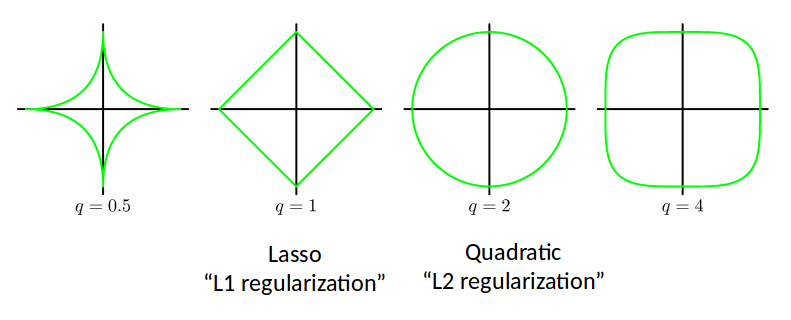
If one is given the following regression problem and face the problem of having too many features, then the immediate thought is to add a regularization term $R(\Xi)$ as $$ \min_{\Xi} \norm{\dot X - \Theta(X)\Xi} + \color{red}{\lambda R(\Xi)} $$ where $\lambda$ is a penalty factor and $R(\Xi)$ could be,
- Frobenius norm $\norm{\Xi}_F$: then we get ridge regression - many coefficients will be small, but non-zero
- L1 norm $\norm{\Xi}_1$: then we get Lasso regression - more coefficients will be exactly zero.
- L0 norm $\norm{\Xi}_0$: then we get the most zeros - but this is a non-convex term and hard to solve.
- In vanilla SINDy, a relatively simple STLSQ (Sequentially Thresholded Least SQuares) algorithm was used.
- STLSQ essentially removes small coefficient iteratively and manually.
- But in the following we present a more recent version of algorithm, Sparse Relaxed Regularized Regression (SR3) [1]
[1] Champion, K., et al., A unified sparse optimization framework to learn parsimonious physics-informed models from data, 2020.
Consider a "relaxed" optimization formulation with an auxiliary variable $W$ $$ \min_{\Xi,W} \frac{1}{2}\norm{\dot X - \Theta(X)\Xi}^2 + \lambda R(W) + \frac{1}{2\nu}\norm{\Xi-W}^2 $$ when $\nu\rightarrow 0$, the formulation reduces to $$ \min_{\Xi} \norm{\dot X - \Theta(X)\Xi} + \lambda R(\Xi) $$
But now,
- The two quadratic parts can be solved in closed-form if $W$ is given
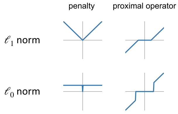
- The regularization term $R(W)$ can be implemented using a technique called the proximal method.
- The idea is that enforcing the regularization on $W$ is equivalent to applying the proximal operator to $W$
- This formulation allows for the addition of constraints, if needed
- One could add physics-informed priors on the model, e.g. identical coefficients due to symmetry, zero coefficients due to skew-symmetry, etc.
Examples of proximal operators:
The algorithm goes as follows
- Pick a penalty parameter $\lambda$, relaxation parameter $\nu$, and number of iterations $N_{itr}$
- Start with a regular least squares solution $$ W^0 = \Theta(X)^+\dot{X} $$
- For $i=1,2,\cdots,N_{itr}$:
- Solve the quadratic part of the problem - for which closed-form solution is available $$ \Xi^k = \min_{\Xi} \frac{1}{2}\norm{\dot X - \Theta(X)\Xi}^2 + \frac{1}{2\nu}\norm{\Xi-W^{k-1}}^2 $$
- Apply the proximal operation. For L0 penalty, this is to simply zero out small coefficients (determined by $\lambda\nu$) $$ W^k = \mathrm{prox}_{\lambda\nu R}(\Xi^k) $$
- Compare the change in truncated coefficients $$ \epsilon = \norm{W^k-W^{k-1}} / \nu $$
- Stop if $\epsilon$ is lower than a user-supplied threshold; otherwise continue
Side note
- See more on proximal gradient method in our notes for Linear Regression - Regularization.
- There are certainly more methods for sparsity enforcement, such as in [1]
[1] Gueho, D., et al., Filtered Integral Formulation of the Sparse Model Identification Problem, 2021.
Try the new optimizer out
# Using the same data
dt, Tf, eps = 0.0001, 1.0, 0.0
x0s = [[1,0], [3,3]]
t_train, x_train = genDataFixPar(dt, Tf, eps, x0s, (OM, MU))
x0t = [[-0.5,-0.5], [-2,3]]
t_test, x_test = genDataFixPar(dt, Tf, eps, x0t, (OM, MU))
opt = ps.SR3(
    threshold=0.8,
    thresholder="l0",
    max_iter=10000,
    tol=1e-10)       # The new optimizer

model_sr3 = ps.SINDy(
    differentiation_method=ps.FiniteDifference(order=2),
    feature_library=ps.PolynomialLibrary(degree=5, include_bias=False),
    optimizer=opt,
    feature_names=["x", "y"])
model_sr3.fit(x_train, t=t_train, multiple_trajectories=True)
print('Fitted coefficients - It is picking out the correct terms!')
model_sr3.print()
Fitted coefficients - It is picking out the correct terms!
(x)' = -10.000 y + 3.992 x^3 + 4.011 x y^2 + -0.998 x^5 + -2.001 x^3 y^2 + -1.003 x y^4
(y)' = 10.000 x + 4.001 x^2 y + 4.002 y^3 + -1.000 x^4 y + -2.001 x^2 y^3 + -1.001 y^5
# Now the test prediction is almost perfect
x_pred = predTrajFixPar(model_sr3, x0t, t_train)
cmpTraj2D(x_test, x_pred, t_train, 2)
Solving [-0.5, -0.5]
Solving [-2, 3]

Denoising the data
The success of the regression relies on the accuracy of the time derivative.
Effect of noise in sample data
# Using the same set up, but now with noise
dt, Tf, eps = 0.0001, 1.0, 0.1
x0s = [[-1.5,1], [2,2], [1,0], [3,3]]
t_train, x_train = genDataFixPar(dt, Tf, eps, x0s, (OM, MU))
# Set zero noise in test data
x0t = [[-2,2], [1,2.5]]
t_test, x_test = genDataFixPar(dt, Tf, 0.0, x0t, (OM, MU))
# Fit the model with customized features
model_noise = ps.SINDy(
    differentiation_method=ps.FiniteDifference(order=2),
    feature_library=clib_lco,
    optimizer=ps.SR3(threshold=0.8, thresholder="l0",
                     max_iter=10000, tol=1e-10),
    feature_names=["x", "y"])
model_noise.fit(x_train, t=t_train, multiple_trajectories=True)
model_noise.print()
print('\nFitted coefficients - even with cheating the fitting fails!')
model_noise.coefficients()
(x)' = 21.635 y + -0.067 xr^2 + -7.913 yr^2
(y)' = 10.791 x + -18.559 y + -0.163 xr^2 + 10.486 yr^2 + -1.451 yr^4

Fitted coefficients - even with cheating the fitting fails!
array([[ 0.0000,  21.6354, -0.0667, -7.9125,  0.0000,  0.0000],
       [ 10.7908, -18.5590, -0.1632,  10.4856,  0.0000, -1.4508]])
# Even the prediction for train trajectories does not work well
x_pred = predTrajFixPar(model_noise, x0s, t_train)
cmpTraj2D(x_train, x_pred, t_train, 2)
Solving [-1.5, 1]
Solving [2, 2]
Solving [1, 0]
Solving [3, 3]

# Another comparison, in quiver plot - clearly the noise creates a problem
cmpPhasePlane((OM,MU), [model_noise], ['Model with noisy data'])

To start with...
There are some simple technique to tackle the data noise. For example,
- Apply classical signal filters, such as Savitzky-Golay, to data before computing the derivative
- Use Fourier method to compute the time derivative,
- Consider the Fourier transform $\hat{X}=\cF(X)$
- Zero out the high-frequency components in $\hat{X}$, which are likely to be noise
- Compute the time derivative as $$ \dot{X} = \cF^{-1}(\mathbb{i}\omega \hat{X}) $$
But certainly there is a lot of tuning work to do - see complaints in [1]
[1] Rudy, S., et al., Data-driven discovery of partial differential equations, 2017.
# Still fitting the model with customized features
# But now with smoothed finite difference for time derivatives
model_smooth = ps.SINDy(
    differentiation_method=ps.SmoothedFiniteDifference(order=2),
    feature_library=clib_lco,
    optimizer=ps.SR3(threshold=0.4, thresholder="l0",
                     max_iter=20000, tol=1e-12),
    feature_names=["x", "y"])
model_smooth.fit(x_train, t=t_train, multiple_trajectories=True)
model_smooth.print()
print('\nFitted coefficients - does not seem to work well!')
model_smooth.coefficients()
(x)' = 4.861 x + -27.096 y + -1.202 xr^2 + 9.029 yr^2 + -1.177 yr^4
(y)' = 7.639 x + 2.659 xr^2 + 1.843 yr^2 + -0.516 xr^4 + -0.458 yr^4

Fitted coefficients - does not seem to work well!
array([[ 4.8613, -27.0956, -1.2017,  9.0287,  0.0000, -1.1770],
       [ 7.6390,  0.0000,  2.6589,  1.8431, -0.5161, -0.4575]])
# Somewhat improved
x_pred = predTrajFixPar(model_smooth, x0s, t_train)
cmpTraj2D(x_train, x_pred, t_train, 2)
Solving [-1.5, 1]
Solving [2, 2]
Solving [1, 0]
Solving [3, 3]

# # But DIVERGES in the second test case
# x_pred = predTrajFixPar(model_smooth, x0t, t_train)
# cmpTraj2D(x_test, x_pred, t_train, 2)
The weak form formulation
Next let's introduce a fancier technique with the understanding that
Differentiating noisy data amplifies noise, but integrating it smoothes out noise
First recall that if one has a series of data points $x_i=x(t_i)$ on grid points $t_I < t_{I+1} < \cdots < t_J$, then the integration of $x(t)$ over $\Omega_t=[t_I,t_J]$ can be approximated as $$ \int_{\Omega_t} x(t) dt \approx \sum_{i=I}^J w_i x_i $$ where the weight $w_i$ depends on the grid points. A typically method is the trapezoidal rule.
Consider noisy data $x_i$ over a time interval $\Omega_t=[t_I,t_J]$, as well as another known smooth function $\phi(t)$ that vanishes at $t=t_I$ and $t=t_J$. Then $$ \int_{\Omega_t} \dot{x} \phi dt = x\phi|_{t_I}^{t_J} - \int_{\Omega_t} x\dot{\phi} dt = - \int_{\Omega_t} x\dot{\phi} dt $$
The last equation is the so-called weak form, which is rooted in functional analysis for PDEs
Then we are able to transfer the difficult derivative on noisy data to a much easier derivative on a known smooth function. Furthermore,
$$ \int_{\Omega_t} x\dot{\phi} dt \approx \sum_{i=I}^J w_i x_i \dot{\phi}(t_i) \equiv -q^T x $$
We can apply the integral and the weak form to the entire system equation, $$ \int_{\Omega_t} \begin{bmatrix} \dot{x}_1 \\ \dot{x}_2 \\ \vdots \\ \dot{x}_N \end{bmatrix} \phi dt = \int_{\Omega_t} \begin{bmatrix} \xi_{11} & \xi_{12} & \cdots & \xi_{1M} \\ \xi_{21} & \xi_{22} & \cdots & \xi_{2M} \\ \vdots & \vdots & \ddots & \vdots \\ \xi_{N1} & \xi_{N2} & \cdots & \xi_{NM} \end{bmatrix} \begin{bmatrix} \theta_1(x) \\ \theta_2(x) \\ \vdots \\ \theta_M(x) \end{bmatrix} \phi dt $$
$$ - \begin{bmatrix} \int_{\Omega_t} x_1 \dot{\phi} dt \\ \int_{\Omega_t} x_2 \dot{\phi} dt \\ \vdots \\ \int_{\Omega_t} x_N \dot{\phi} dt \end{bmatrix} = \begin{bmatrix} \xi_{11} & \xi_{12} & \cdots & \xi_{1M} \\ \xi_{21} & \xi_{22} & \cdots & \xi_{2M} \\ \vdots & \vdots & \ddots & \vdots \\ \xi_{N1} & \xi_{N2} & \cdots & \xi_{NM} \end{bmatrix} \begin{bmatrix} \int_{\Omega_t} \theta_1(x) \phi dt \\ \int_{\Omega_t} \theta_2(x) \phi dt \\ \vdots \\ \int_{\Omega_t} \theta_M(x) \phi dt \end{bmatrix} $$ where each of the integral can be numerically evaluated, without much impact from noise.
Consider a series of $N_\Omega$ intervals $\Omega_i$ and $N_\phi$ functions $\phi_j$, a linear system of equations is formed and denoted $$ \dot{q}_{i,j}=\Xi^Tq_{i,j} $$ These equations can be assembled in the familiar least squares form $$ \min_{\Xi} \norm{\dot{Q} - Q\Xi} $$ where $Q^T=[q_{1,1},q_{1,2},\cdots,q_{1,N_\phi},\cdots,q_{N_\Omega,N_\phi}]$, and similarly for $\dot{Q}^T$.
Side note
- Nothing prevents the weak formulation to be applied to partial differential equations (PDEs). In fact, discovery of PDEs from noisy data is how initially this method was developed for. See [1] for more details.
- Another approach recommended for tackling noise along with weak form is the ensemble method. For example, one can subsample a noisy trajectory to create multiple, sparser trajectories, for each of which the SINDy model is trained - so that one gets an ensemble of models. Finally, one chooses, e.g., the average or the median of the models for prediction. Similarly one can do ensemble for the features, or both. See [2] for more details.
[1] Reinbold, P., et al., Using noisy or incomplete data to discover models of spatiotemporal dynamics, 2020.
[2] PySINDy Documentation: Ensembling Feature Overview
Try the weak form out
# Again we use PySINDy implementation
pts, K = 400, 400
ode_lib = ps.WeakPDELibrary(
    library_functions=clib_func, function_names=clib_name, spatiotemporal_grid=t_train,
    include_bias=False, is_uniform=True, num_pts_per_domain=pts, K=K)
opt = ps.SR3(threshold=0.4, thresholder="l0", max_iter=60000, tol=1e-12)

model = ps.SINDy(feature_library=ode_lib, optimizer=opt, feature_names=["x", "y"])
model.fit(x_train, multiple_trajectories=True)
model_weak = wsWrapper(model, clib_lco, opt, x_train, t_train)
model_weak.print()
print('\nFitted coefficients - cannot say the coefficients are the most accurate')
model_weak.coefficients()
(x)' = -21.735 y + 2.238 xr^2 + 5.490 yr^2 + -0.559 xr^4 + -0.630 yr^4
(y)' = 10.791 x + -18.559 y + -0.163 xr^2 + 10.486 yr^2 + -1.451 yr^4

Fitted coefficients - cannot say the coefficients are the most accurate
/Users/daninghuang/Library/Python/3.8/lib/python/site-packages/pysindy/optimizers/sr3.py:388: ConvergenceWarning: SR3._reduce did not converge after 60000 iterations.
  warnings.warn(
array([[ 0.0000, -21.7348,  2.2385,  5.4900, -0.5588, -0.6299],
       [ 10.7908, -18.5590, -0.1632,  10.4856,  0.0000, -1.4508]])
# We lost one training case...
x_pred = predTrajFixPar(model_weak, x0s, t_train)
cmpTraj2D(x_train, x_pred, t_train, 2)
Solving [-1.5, 1]
Solving [2, 2]
Solving [1, 0]
Solving [3, 3]

# But the test cases seem to work really well
x_pred = predTrajFixPar(model_weak, x0t, t_train)
cmpTraj2D(x_test, x_pred, t_train, 2)
Solving [-2, 2]
Solving [1, 2.5]

# A closer look at the phase plane - note the catastrophic diverging region in the model with smoothed FD
cmpPhasePlane((OM,MU), [model_smooth, model_weak], ['Smoothed FD', 'Weak form'])

Handling parameters
Finally, we look at an extended problem with system parameters $$ \dot{x}=F(x,\mu) $$ We have been keeping $\mu$ fixed in previous examples.
How about finding a model that works for a range of $\mu$'s?
It is easy
Using the previous example, we can simply modify the model to be learned as $$ \begin{bmatrix} \dot{x} \\ \dot{y} \\ \color{red}{\dot{\mu}} \end{bmatrix} = \begin{bmatrix} -\omega y - x r^2(r^2-\mu) \\ \omega x - y r^2(r^2-\mu) \\ \color{red}{0}\end{bmatrix} $$ so that $\mu$ behaves as if a state and can appear in the system function as a variable like $x$ and $y$.
The rest is then just like regular SINDy
However be careful that the order of features should increase.
# Now we generate a new dataset
dt, Tf, eps = 0.0001, 2.0, 0.0
# Training: mu = -2, -1, 0, 1, 2
x0s = [[-1.5,1], [2,2], [1,0], [3,3]]
args = [(OM,-2), (OM,-1), (OM,0), (OM,1), (OM,2)]
inps = [(_a[1],) for _a in args]
t_train, x_train = genDataMultiPar(dt, Tf, eps, x0s, args, 1)
# Test: mu = -2.5, -1.5, -0.5, 0.5, 1.5, 2.5
x0t = [[-2,2], [1,2.5]]
argt = [(OM,-2.5), (OM,-1.5), (OM,-0.5), (OM,0.5), (OM,1.5), (OM,2.5)]
inpt = [(_a[1],) for _a in argt]
t_test, x_test = genDataMultiPar(dt, Tf, eps, x0t, argt, 1)
optimizer = ps.SR3(
    threshold=1.0,
    thresholder="l0",
    max_iter=1000,
    tol=1e-10)
library = ps.PolynomialLibrary(degree=6, include_bias=False)
model = ps.SINDy(optimizer=optimizer, feature_library=library, feature_names=['x', 'y', 'u'])
model.fit(x_train, t=t_train, multiple_trajectories=True, quiet=True)
model.print()
# Numbers are looking familiar and the last term is correctly zero.
(x)' = -10.086 y + 1.686 x^3 u + -1.560 x^5 + -1.986 x^3 y^2 + -0.476 x y^4
(y)' = 10.064 x + 0.752 x^2 y u + 1.103 y^3 u + -2.980 x^2 y^3 + -0.972 y^5
(u)' = 0.000
# Comparing the trajectories in 3D - they look identical!
# Also note that some of the test cases are BEYOND the training cases
cmpTraj3D(x_test, x_pred, 2)

Side note
There are many more variants and applications of the SINDy algorithm. Just naming a few:
- To handle implicit ODEs - see [1]
- To handle control inputs - see [2]
- See [3] for a recent summary of extensions and watch PySINDy@github for updates.
[1] Kaheman, K., et al., SINDy-PI: a robust algorithm for parallel implicit sparse identification of nonlinear dynamics, 2020.
[2] Brunton, S., et al., Sparse Identification of Nonlinear Dynamics with Control (SINDYc), 2016.
[3] Kaptanoglu, A., et al., PySINDy: A comprehensive Python package for robust sparse system identification, 2022.