TODAY: Gaussian Process Regression - I
- Historical background: kriging
- Multivariate correlation
References
- GPML Chps. 1, 2, 4
- DACE Toolbox Manual
"Kriging" model by Danie G. Krige
Danie Gerhardus Krige (26 August 1919 – 3 March 2013), South African statistician and mining engineer who pioneered the field of geostatistics. Inventor of kriging.

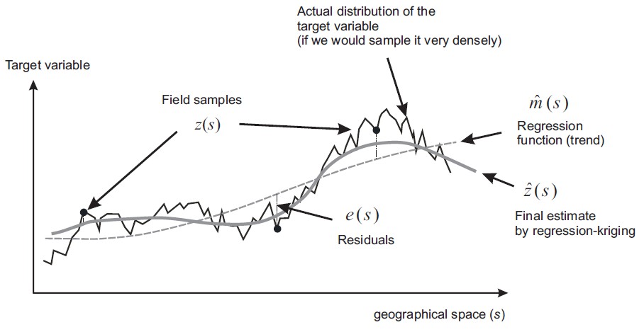
- Capture the global trend of a dataset, such that the error behaves like white noise.
- But now the noise is location-depedent.
A non-parametric model uses all the training data to do predictions. In contrast, a parametric model obtains its "parameters" from the training data before prediction, and only uses those parameters for prediction.
The non-parametric model based on Gaussian process (GPR) has been around for quite a while. It has deep connections to methods such as radial basis function network (RBFN). In geostatistics, and later in the field of engineering, the method is called kriging. The GPR with explicit mean function is also called generalized least squares (GLS). There are two good properties of GPR. First, GPR can handle the noise in the sample data. Second, the model not only provides the interpolated value, but also the uncertainty of the prediction. These properties can be particularly useful in engineering applications, e.g. for optimization and uncertainty quantification.
The idea of GPR is simple. It assumes that all data points are sampled from a Gaussian process, and therefore these points subject to a joint Gaussian distribution. The new data point should subject to a Gaussian distribution as well, determined by the training data. In that Gaussian distribution, the mean becomes the prediction, and the variance becomes the error estimation. In this module, the derivation of GPR will be presented, with some discussion in computational aspects.
Correlation and Covariance
Covariance function
# Spatial correlation between Gaussian samples at different locations
a = [0.0, 0.0]
x, RV, KS = genGP(5,     # Number of sampling points
                  0.05,  # Length scale in a SE correlation term
                  a,     # Coefficients of second-order polynomial
                  1000)  # Number of GP realizations
plt.figure()
plt.imshow(KS)
plt.colorbar()
_=pltCorr(x, RV)
_=pltGP(x, RV, a,
        bnd=True,             # Plot error bounds
        smp=True)


# Realizations over a set of sampling points
a = [10.0, 0.0]
x, RV, _ = genGP(200,           # Number of sampling points
                 0.0025,        # Length scale in a SE correlation term
                 a,             # Coefficients of second-order polynomial
                 1000)          # Number of GP realizations
_=pltGP(x, RV, a,
        bnd=True,             # Plot error bounds
        smp=True)             # Highlight three samples and plot the mean
