TODAY: Gaussian Process Regression - III
- Monte Carlo simulation
- Basics of Markov chain
- Metropolis-Hastings sampling
- Gibbs sampling
References
- [PRML] Chp. 11
- twiecki.io
Model Selection Revisited
Model selection refers to two tasks of interest:
- Task 1: Given a model $\cM$ with hyperparameters $\theta$ and a dataset $\cD$, find $\theta$ such that $\cM$ fits $\cD$ the best.
- e.g. $\cM$: A GPR with a correlation function; $\theta$: Length scales in the correlation function.
- Task 2: Given several models $\cM_1, \cM_2, \cdots$ and a dataset $\cD$, find $\cM_j$ that fits $\cD$ the best.
- e.g. GPR's with different correlation/trend functions.
- For Task 1, one can determine $\theta$ by maximizing the likelihood
$$
\theta_{MLE} = \mathrm{arg\ max}_\theta p(\cD|\theta,\cM)
$$
As disscused in the previous lectures for GPR.
- For Task 2, one could use cross validation, or certain information criteria, to assess the fitness of different models.
- For Task 1, one could also employ a Bayesian approach by assigning priors to $\theta$, and evaluate the posterior,
$$
p(\theta|\cD,\cM)=\frac{p(\cD|\theta,\cM)p(\theta|\cM)}{p(\cD|\cM)}\propto p(\cD|\theta,\cM)p(\theta|\cM)
$$
- The posterior $p(\theta|\cD,\cM)$ provides an estimation of $\theta$ given the dataset and model, with a confidence bound.
- For Task 2, the evidence $p(\cD|\cM)$ provides a "rigorous" and quantitative assessment of the model fitness.
Sounds like better than MLE+CV?
Two issues with the Bayesian approach:
- For Task 1, the posterior $p(\theta|\cD,\cM)$ typically do not have a closed-form expression. For example, in GPR
- $p(\cD|\theta,\cM)$ is typically Gaussian - but in some fancier models it is non-Gaussian
- $p(\theta|\cM)$ could be a Beta distribution, if $\theta$ are the length scales (positive valued)
- As a result, for Task 2, it is non-trivial to evaluate the integral for the evidence: $$ p(\cD|\cM) = \int_\Theta p(\cD|\theta,\cM)p(\theta|\cM) d\theta $$
Solution - Markov chain Monte Carlo algorithm
- A procedure to generate samples $\{\theta^{(i)}\}_{i=1}^N$ from the posterior distribution $p(\theta|\cD,\cM)\propto p(\cD|\theta,\cM)p(\theta|\cM)$.
- Then one can use a histogram, or a kernel density estimation, to approximate the posterior distribution.
- With the posterior distribution, you can locate the best parameters.
- You can also evaluate the evidence to assess the fitness of the model.
- Challenge: How to generate samples satisfying an unnormalized distribution $p(\cD|\theta,\cM)p(\theta|\cM)$?
Monte Carlo Simulation
- "Integration by Darts": $$ \int f(\vz)p(\vz) d\vz \approx \frac{1}{L}\sum_{l=1}^L f(\vz^{(l)}) $$
where the samples $\vz^{(l)}$ are drawn from $p(\vz)$.
For the evidence, one can draw $\theta^{(i)}$ from $p(\theta|\cM)$, and do: $$ p(\cD|\cM) = \int_\Theta p(\cD|\theta,\cM)p(\theta|\cM) d\theta \approx \frac{1}{N}\sum_{i=1}^N p(\cD|\theta^{(i)},\cM) $$
So the issue for Task 2 is somehow resolved.
# Estimating area of circle by MC.
# Very simple as p(z) is a uniform distribution defined on unit square.
# and f(z)=1 in circle and f(z)=0 out of circle.

N = 10000
s = np.random.uniform(size=(2,N))
x, y = s[0], s[1]
r2 = (x-0.5)**2 + (y-0.5)**2
m = r2 <= 0.25

f = plt.figure(figsize=(6,4))
plt.plot(x[m], y[m], 'b.')
plt.plot(x[~m], y[~m], 'r.')
plt.title('Area: Accurate = {0:4.3f}, Approx. = {1:4.3f}'.format(np.pi*0.25, np.sum(m)/float(N)))
a = plt.axis('equal')

area = np.cumsum(m)/np.arange(1.0,N+1.0)
f = plt.figure(figsize=(6,4))
_=plt.loglog(np.abs(area-np.pi*0.25))

Importance Sampling
For a distribution $p(\vz)$ that is hard to sample, one can introduce a simpler distribution $q(\vz)$, $$ \int f(\vz)p(\vz) d\vz = \int f(\vz)\frac{p(\vz)}{q(\vz)}q(\vz) d\vz \approx \frac{1}{L}\sum_{l=1}^L f(\vz^{(l)})\frac{p(\vz^{(l)})}{q(\vz^{(l)})} $$
But maybe the target distribution cannot even be easily normalized, one can do, $$ \int f(\vz)p(\vz) d\vz \approx \frac{Z_q}{Z_p} \frac{1}{L}\sum_{l=1}^L \tilde{r}^{(l)}f(\vz^{(l)}) $$ where $Z_q$ and $Z_p$ are normalizing factors for $\tilde{q}$ and $\tilde{p}$, respectively, and $$ \tilde{r}^{(l)}=\frac{\tilde{p}(\vz^{(l)})}{\tilde{q}(\vz^{(l)})} $$
But one also has, $$ \frac{Z_p}{Z_q} = \int \frac{\tilde{p}(\vz)}{\tilde{q}(\vz)}q(\vz) d\vz \approx \frac{1}{L}\sum_{l=1}^L \tilde{r}^{(l)} $$ so the integral simplifies to $$ \int f(\vz)p(\vz) d\vz \approx \sum_{l=1}^L w^{(l)}f(\vz^{(l)}),\quad w^{(l)}=\tilde{r}^{(l)}\left/\left(\sum_l \tilde{r}^{(l)}\right)\right. $$
Accept-Reject Sampling
Given a difficult, maybe unnormalized, distribution $p(\vz)$:
- Pick $q(\vz)$ and a constant $k$ such that $p(\vz)<kq(\vz)$.
- Sample $\vz_0$ from $q(\vz)$
- Sample $u\sim \mathrm{Uniform}[0,kq(\vz_0)]$
- If $u\leq p(\vz_0)$, accept $\vz_0$, otherwise reject.
The samples of $p(\vz)$ is represented by a carefully selected subset of samples of $q(\vz)$.
f = plt.figure(figsize=(6,4))
plt.plot(x, g, 'b-', label='g(x)')
plt.plot(x, c*g, 'b--', label='c*g(x)')
plt.plot(x, y, 'k-', label='f(x)')
plt.hist(ss_all, bins=50, density=True, color='y', label='All samples')
plt.hist(ss_acc, bins=50, density=True, color='r', label='Accepted')
plt.legend()
_=plt.title('# of Samples: {0}'.format(Nsmp))

Markov Models
Uses material from [MLAPP]
Markov Models
A Markov chain is a series of random variables $X_1, \dots, X_N$ satisfying the Markov property:
The future is independent of the past, given the present. $$ p(x_n | x_1, \dots, x_{n-1}) = p(x_n | x_{n-1}) $$
A chain is stationary if the transition probabilities do not change with time.
Markov Models: Joint Distribution
If a sequence has the Markov property, then the joint distribution factorizes according to $$ p(x_1, \dots, x_N) = p(x_1) \prod_{n=2}^N p(x_n | x_{n-1}) $$
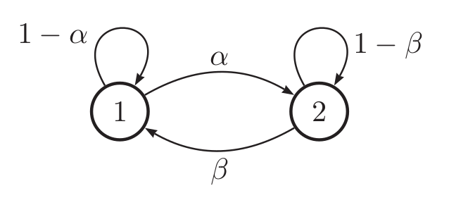
Markov Models: Transition Matrix
Suppose $X_t \in \{1,\dots,K\}$ is discrete. Then, a stationary chain with $N$ states can be described by a transition matrix, $A \in \bR^{N \times N}$ where $$ a_{ij} = p(X_t=j \mid X_{t-1}=i) $$
is the probability of transitioning from state $i$ to $j$.
Each row sums to one, $\sum_{j=1}^K A_{ij} = 1$, so $A$ is a row-stochastic matrix.
Markov Models: State Vectors
Consider a row vector $x_t \in \bR^{K \times 1}$ with entries $x_{tj} = p(X_t = j)$. Then, $$ \begin{align} p(X_t = j) &= \sum_{i=1}^K p(X_t = j \mid X_{t-1} = i) p(X_{t-1} = i) \\ &= \sum_{i=1}^K A_{ij} x_{t-1,i} \\ \end{align} $$ Therefore, we conclude $x_t = x_{t-1} A$. Note $\sum_{j=1}^K x_{tj} = 1$.
Markov Models: Matrix Powers
Since $x_t = x_{t-1} A$, this suggests that in general, $$ x_{t} = x_{t-1} A = x_{t-2} A^2 = \cdots x_{0} A^t $$ If we know the initial state probabilities $x_0$, we can find the probabilities of landing in any state at time $t > 0$.
Example: Weather
Suppose the weather is either $R=\text{Rainy}$ or $S=\text{Sunny}$, $$ A = \begin{bmatrix} 0.9 & 0.1 \\ 0.5 & 0.5 \end{bmatrix} $$
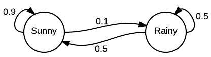
Example: Weather
Suppose today is sunny, $x_0 = \begin{bmatrix} 1 & 0 \end{bmatrix}$. We can predict tomorrow's weather, $$ x_1 = x_0 A = \begin{bmatrix} 0.9 & 0.1 \end{bmatrix} $$ The weather over the next several days will be $$ \begin{align} x_2 &= x_1 A = \begin{bmatrix} 0.86 & 0.14 \end{bmatrix} \\ x_3 &= x_2 A = \begin{bmatrix} 0.844 & 0.156 \end{bmatrix} \\ x_4 &= x_3 A = \begin{bmatrix} 0.8376 & 0.1624 \end{bmatrix} \end{align} $$
Question: What happens to $x_0 A^n$ as $n \rightarrow \infty$?
Markov Chains: Stationary Distribution
If we ever reach a stage $x$ where $$ x = xA $$ then we have reached the stationary distribution of the chain.
- To find $x=v^T$, solve the eigenvalue problem $A^T v = v$
- Under certain conditions, the limiting distribution $\lim_{n \rightarrow \infty} x_0 A^n = x$
- Stationary distribution $x$ does not depend on the starting state $x_0$
f = plt.figure(figsize=(6,4))
for _s in history:
    plt.plot(_s[0])
plt.xlabel('No. of transitions')
_=plt.ylabel('Probability of Sunny')

MCMC
Detailed Balance
- A stationary distribution $\pi(x)$ satisfies the detailed balance condition: $$ \pi(i)P(i,j) = \pi(j)P(j,i) $$
Proof: $$ \sum\limits_{i=1}^{\infty}\pi(i)P(i,j) = \sum\limits_{i=1}^{\infty} \pi(j)P(j,i) = \pi(j)\sum\limits_{i=1}^{\infty} P(j,i) = \pi(j) $$ i.e. $\pi P = \pi$
- So it is possible to find the transition matrix from the stationary distribution, which could be the distribution to be sampled.
- Yet it is nontrivial to satisfy detailed balance. With a random guess $Q(x,y)$, one gets $$ \pi(i)Q(i,j) \neq \pi(j)Q(j,i) $$
Similar to the idea from accept-reject sampling, let's introduce a correction $\alpha(i,j)$, called acceptance rate, such that: $$ \pi(i)Q(i,j)\alpha(i,j) = \pi(j)Q(j,i)\alpha(j,i) $$
To make the above happen, $\alpha$ should satisfy, $$ \begin{align} \alpha(i,j) &= \pi(j)Q(j,i) \\ \alpha(j,i) &= \pi(i)Q(i,j) \end{align} $$
And we have, $$ P(i,j) = Q(i,j)\alpha(i,j) $$
Basic MCMC
We do a loop of sampling:
- Sample $x_*$ from $Q(x,x_{t-1})$
- Sample $u \sim \mathrm{Uniform}[0,1]$
- If $u < \alpha(x_{t-1},x_{*}) = \pi(x_{*})Q(x_{*},x_{t-1})$, then $x_t= x_{*}$, else $x_t= x_{t-1}$ The set of samples $\{x_0, x_1, \cdots, x_n\}$ are then the MCMC samples.
Issue: $\alpha$ could be low, resulting in many rejected samples.
Metropolis-Hastings Sampling
Note that $\alpha$ is insusceptible to scales: $$ \pi(i)Q(i,j)\alpha(i,j) = \pi(j)Q(j,i)\alpha(j,i) \ \Leftrightarrow\ \pi(i)Q(i,j)(5\alpha(i,j)) = \pi(j)Q(j,i)(5\alpha(j,i)) $$
So one could define $$ \alpha(i,j) = \min\left\{ \frac{\pi(j)Q(j,i)}{\pi(i)Q(i,j)},1 \right\} $$ to obtain an acceptance rate $\alpha$ that is maximum possible.
Proof that the definition works: $$ \begin{align} &\quad \pi(i)Q(i,j)\alpha(i,j) \\ &= \pi(i)Q(i,j)\min\left\{ \frac{\pi(j)Q(j,i)}{\pi(i)Q(i,j)},1 \right\} \\ &= \min\{\pi(j)Q(j,i), \pi(i)Q(i,j)\} = \pi(j)Q(j,i) \min\left\{ 1,\frac{\pi(i)Q(i,j)}{\pi(j)Q(j,i)} \right\} \\ &= \pi(j)Q(j,i)\alpha(j,i) \end{align} $$
f = plt.figure(figsize=(6,4))
plt.hist(p, 50, density=True, facecolor='red', alpha=0.7, label='Sample PDF')
plt.scatter(p, [56.818*targetPDF(_) for _ in p], label='Target PDF')
_=plt.legend()

Issues
Curse of dimensionality:
- For example, volume of high prod. region of high-dim Gaussian ~ $\sigma^{-D}$
- Computational cost: $\frac{\pi(j)Q(j,i)}{\pi(i)Q(i,j)}$, and the proposed sample could be rejected
- Sometimes it is even hard to get joint distribution.
One of the cures is the Gibbs sampling method.
Gibbs Sampling
Detailed balance requires: $$ \pi(i)P(i,j) = \pi(j)P(j,i) $$
Consider a 2D case $\pi(x_1,x_2)$ and two points: $A(x_1^{(1)},x_2^{(1)})$ and $B(x_1^{(1)},x_2^{(2)})$. One has
$$ \begin{align} \pi(x_1^{(1)},x_2^{(1)}) \pi(x_2^{(2)} | x_1^{(1)}) &= \pi(x_1^{(1)})\pi(x_2^{(1)}|x_1^{(1)}) \pi(x_2^{(2)} | x_1^{(1)}) \\ \pi(x_1^{(1)},x_2^{(2)}) \pi(x_2^{(1)} | x_1^{(1)}) &= \pi(x_1^{(1)}) \pi(x_2^{(2)} | x_1^{(1)})\pi(x_2^{(1)}|x_1^{(1)}) \end{align} $$This is saying: $$ \begin{align} \pi(x_1^{(1)},x_2^{(1)}) \pi(x_2^{(2)} | x_1^{(1)}) &= \pi(x_1^{(1)},x_2^{(2)}) \pi(x_2^{(1)} | x_1^{(1)}) \\ \mbox{or } \pi(A) \pi(x_2^{(2)} | x_1^{(1)}) &= \pi(B) \pi(x_2^{(1)} | x_1^{(1)}) \end{align} $$
Or, $\pi(x_2| x_1^{(1)})$ can be used to satisfy detailed balance of Markov chain!
Algorithm - 2D version
- Given stationary distribution $\pi(x_1,x_2)$
- Set initial states $x_1^{(0)}$ and $x_2^{(0)}$
- Loop for sampling:
- (a) Sample $x_2^{t+1}$ from $P(x_2|x_1^{(t)})$
- (b) Sample $x_1^{t+1}$ from $P(x_1|x_2^{(t)})$
Then, samples are generated from rotating the coordinate axes $$ (x_1^{(1)}, x_2^{(1)}) \to (x_1^{(1)}, x_2^{(2)}) \to (x_1^{(2)}, x_2^{(2)}) \to ... \to (x_1^{(n)}, x_2^{(n)}) $$
f = plt.figure(figsize=(6,4))
plt.hist(p[0], 50, density=True, facecolor='green', alpha=0.5, label='x')
plt.hist(p[1], 50, density=True, facecolor='red', alpha=0.5, label='y')
_=plt.legend()

Nb = 1000
Ng = 101
x = np.linspace(2, 8, Ng)
y = np.linspace(-7, 5, Ng)
X, Y = np.meshgrid(x, y)
Z = target.pdf(np.vstack([X.reshape(-1), Y.reshape(-1)]).T).reshape(Ng, Ng)
f = plt.figure(figsize=(6,4))
plt.scatter(p[0][Nb:], p[1][Nb:], c=p[2][Nb:])
_=plt.contour(X, Y, Z, colors='w', linewidth=2)

Nb = 1000
M1 = np.mean(p[0][Nb:])
M2 = np.mean(p[1][Nb:])
dx = p[0][Nb:]-M1
dy = p[1][Nb:]-M2
S1 = np.mean(dx**2)
S2 = np.mean(dy**2)
RR = np.mean(dx*dy)
print([M1, M2, S1, S2, RR])
[4.968675138645328, -1.023543892624309, 1.0023609697090448, 4.0025096384248515, 1.0018483992282012]
There are many other methods
One example - auxiliary variable method:
- Introduce a new variable $\vu$, $\vz, \vu\sim p(\vz, \vu)$, so that $$ \int f(\vz)p(\vz)d\vz = \int\int f(\vz)p(\vz,\vu)d\vz d\vu = \frac{1}{N}\sum_{i=1}^N f(x^{(i)}) $$
- Efficient if $p(\vz|\vu)$ or $p(\vu|\vz)$ is easy to sample, or if $p(\vz, \vu)$ is easy to explore.
One specific method is Hamiltonian Monte Carlo
- Let $p(\vz) \propto \exp[-E(\vz)]$, and $$ p(\vz, \vu) \propto \exp[-E(\vz)]\exp(-\vu^T\vu/2)\equiv \exp[-H(\vz,\vu)] $$
- $E(\vz)$ and $\frac{1}{2}\vu^T\vu$ can be considered potential and kinetic energy, respectively. Due to energy conservation, $$ p(\vz,\vu) = p(\vz',\vu') $$
- So one can solve Hamitonian dynamics to do sampling!
- A practical variant: HMC with No U-Turns Sampling (NUTS)
- A challenge: Hamitonian dynamics requires the evaluation of $\frac{\partial E}{\partial \vz}$ - not always available.
- Not a problem for gradient-enabled frameworks, e.g. TensorFlow, pyTorch, FluxML, etc.