$$ \newcommand{\GP}{\mathcal{GP}} \newcommand{\bR}{\mathbb{R}} \newcommand{\cD}{\mathcal{D}} \newcommand{\cL}{\mathcal{L}} \newcommand{\cN}{\mathcal{N}} \newcommand{\vH}{\mathbf{H}} \newcommand{\vI}{\mathbf{I}} \newcommand{\vK}{\mathbf{K}} \newcommand{\vL}{\mathbf{L}} \newcommand{\vM}{\mathbf{M}} \newcommand{\vO}{\mathbf{O}} \newcommand{\vQ}{\mathbf{Q}} \newcommand{\vV}{\mathbf{V}} \newcommand{\vX}{\mathbf{X}} \newcommand{\vY}{\mathbf{Y}} \newcommand{\vb}{\mathbf{b}} \newcommand{\vf}{\mathbf{f}} \newcommand{\vg}{\mathbf{g}} \newcommand{\vm}{\mathbf{m}} \newcommand{\vv}{\mathbf{v}} \newcommand{\vx}{\mathbf{x}} \newcommand{\vy}{\mathbf{y}} \newcommand{\sns}{\sigma_n^2} \newcommand{\Dx}{{\nabla\vx}} $$
Limitations of "vanilla" GPR
What we learned so far: $$ \begin{align} \vm_p &= \vm_u + \vK_{us}\vK_y^{-1}(\vy_s-\vm_s) \\ \vK_p &= \vK_{uu} - \vK_{us}\vK_y^{-1}\vK_{su} \end{align} $$
- Non-parametric & Dense: Prediction requires using the entire dataset.
- High computational cost:
- Training $O(N^3)$
- Prediction - mean $O(N)$ and variance $O(N^2)$.
Challenges in large dataset
At least two cases:
- Case I: A large dataset is available to GPR, e.g.,
- from experimental high-frequency measurements or sensor data with high frame rate.
- Dataset given as is
- Case II: A large dataset is needed to approximate a function using GPR, because
- Complex landscape, and dense sampling required.
- High-dimensional parameter space, and sufficient sampling required.
- Got to choose where and what to sample for dataset
Case I: Directly Tackling (given) Large Dataset
Basic idea: Reduce the effective sample size $N$ in the model.
Three typical strategies:
- Subset of dataset: Choose a partial set of data points to represent the whole dataset.
- e.g., by greedy approach, but might be suboptimal.
- Low-rank approximation: Replace covariance matrices by
$$
\vK = \vV\vV^T,\quad \vV\in\bR^{N\times M},\quad M\ll N
$$
so that the cost reduces from $O(N^2)$ to $O(MN)$.
- Potential danger of degeneracy: predicting zeros when out-of-distribution (i.e., away from training data).
Type-II example - Nyström method
We choose $M$ samples from the dataset, and let $$ \vK_N \approx \vQ_N = \vK_{NM}\vK_M^{-1}\vK_{MN} $$ which is equivalent to an approximation of the kernel, or subset of regressors (SR), $$ k(\vx,\vx') \approx Q(\vx,\vx') = k(\vx,\vx_M)\vK_M^{-1}k(\vx_M,\vx') $$ This way $\vm_p$ and $\vK_p$ can be simplified using the matrix inversion lemma $$ \begin{align} \vm_p &= \vm_u + \vQ_{us}\vQ_y^{-1}(\vy_s-\vm_s) \\ \vK_p &= \vQ_{uu} - \vQ_{us}\vQ_y^{-1}\vQ_{su} \end{align} $$ where $\vQ_y=\vQ_N+\sns\vI$. However, during prediction, as input points move away from the $M$ samples, $\vK_{MN}$, and thus the variance, will be close to zero.
Comparison of several GP approximations from Snel2008.
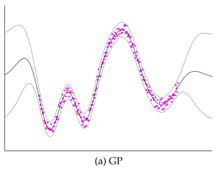
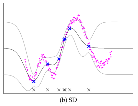
- Subset of Dataset (SD): Choosing a subset of data (input+output); discarding everything else
- Mismatch in many locations
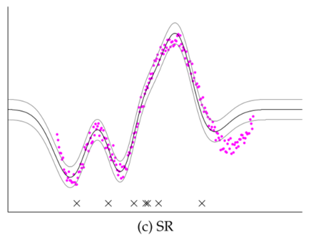
- Subset of Regressors (SR/Nystrom): Choosing a subset of inputs, but retain all outputs
- Unrealistically low variance
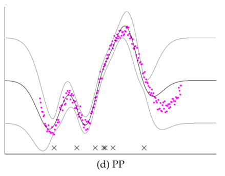
- Projected Process (PP): A fix to SR; using full-rank covariance in prediction. See detailed definition in skipped material.
- Might face challenge in low-noise case.
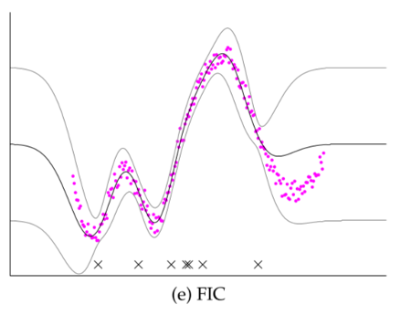
- Fully Independent Conditional (FIC): Even better - got to optimize the subset of inputs, or even use "fake" (but better) inputs.
- See detailed derivations in skipped material.
Historical Note
One interesting approach is the relevance vector machine (RVM). It applies the idea of automatic relevance determination (ARD) and finds the training data point that is of the most "relevance" to the model. Subsequently, a kernel is constructed from these "relevance vectors" to form the final prediction model. Due to the construction of the kernel, RVM is a degenerate GP, which is criticized in Rasm2005. A fun fact of RVM is that its 2001 version algorithm is patented, and partially discouraged its integration into some mainstream packages. Note that its faster, 2003 version of algorithm is not patented, though. One good Python implementation of RVM can be found here.
Another approach of the second type is the GPR with pseudo-inputs Snel2008, or termed fully independent training conditional (FITC). This approach determines a set of points from the training data, not necessarily the points in the dataset itself, and generates the GPR over these "pseudo inputs". The GP is still non-degenerate, but $N$ can be significantly reduced, sometimes by two orders of magnitudes. Yet the prediction is not deteriorated by much.
A Unifying View for Sparse GPR - Skip in class
(From [Quin2005])
The model $$ \vy = \vf + \epsilon $$
- Two types of variables: Observed noisy output $\vy$, Underlying noise-free latent output $\vf$
- Noise $\epsilon\sim\cN(0,\sns)$ (additive and independent)
The predictive model for noisy data $\vy_s$ and desired noise-free output $\vf_u$, $$ \begin{aligned} p(\vf_u|\vy_s) &= \int p(\vf_s,\vf_u|\vy_s) d\vf_s \\ &= \int \frac{p(\vy_s|\vf_s,\vf_u)p(\vf_s,\vf_u)}{p(\vy_s)} d\vf_s \\ &= \frac{1}{p(\vy_s)} \int p(\vy_s|\vf_s)p(\vf_s,\vf_u) d\vf_s \\ \end{aligned} $$
- $p(\vy_s)$ is a normalizing factor and not computed explicitly.
- $p(\vf_s,\vf_u)$ is where the large dense covariance matrix is introduced, and will be simplified next.
Inducing points
Consider additional inducing points $\vf_i$ sampled from the same GP governing $\vf_s$ and $\vf_u$. Then, $$ \vf_i\sim\cN(\vm_i,\vK_{ii}),\quad\text{and}\quad p(\vf_s,\vf_u) = \int p(\vf_s,\vf_u,\vf_i) d\vf_i = \int p(\vf_s,\vf_u|\vf_i)p(\vf_i) d\vf_i $$
Next introduce simplifications: $\vf_s$ and $\vf_u$ are conditionally independent given $\vf_i$, $$ p(\vf_s,\vf_u) \approx q(\vf_s,\vf_u) = \int q(\vf_s|\vf_i) q(\vf_u|\vf_i) p(\vf_i) d\vf_i $$
- This means to predict $\vf_u$, one only needs $\vf_i$ instead of the large set of $\vf_s$.
As a reference, the exact forms of the conditionals and the covariance matrix are, $$ \left\{ \begin{aligned} \vf_s|\vf_i &\sim \cN(\vm_s+\vK_{si}\vK_{ii}^{-1}(\vf_i-\vm_i), \vK_{ss}-\vQ_{ss}) \\ \vf_u|\vf_i &\sim \cN(\vm_u+\vK_{ui}\vK_{ii}^{-1}(\vf_i-\vm_i), \vK_{uu}-\vQ_{uu}) \end{aligned} \right. \quad\vK= \begin{bmatrix} \vK_{ss} & \vK_{su} \\ \vK_{us} & \vK_{uu} \end{bmatrix} $$ where $\vQ_{ab}=\vK_{ai}\vK_{ii}^{-1}\vK_{ib}$.
Approximations
Under the above framework, all the approximations are actually simplifying or approximating the term $\vK_{**}-\vQ_{**}$.
Example 1: Low-rank approximation approach, SR: $$ \left\{ \begin{aligned} \vf_s|\vf_i &\sim \cN(\vm_s+\vK_{si}\vK_{ii}^{-1}(\vf_i-\vm_i), \vO) \\ \vf_u|\vf_i &\sim \cN(\vm_u+\vK_{ui}\vK_{ii}^{-1}(\vf_i-\vm_i), \vO) \end{aligned} \right. \quad\vK= \begin{bmatrix} \vQ_{ss} & \vQ_{su} \\ \vQ_{us} & \vQ_{uu} \end{bmatrix} $$
- The covariance matrices are neglected and the "distributions" become deterministic
- Also called Deterministic Inducing Conditional (DIC) in [Quin2005].
- The zero covariance matrix is exactly the cause of the zero error estimation in this type of approach.
Example 2: Another similar, but better, approximation is called projected process (PP): $$ \vK= \begin{bmatrix} \vQ_{ss} & \vQ_{su} \\ \vQ_{us} & \vK_{uu} \end{bmatrix} $$
- In regions away from the dataset, the variance no longer becomes zero.
- However, challenge in low-noise dataset, see [Quin2005] for more discussion.
Example 3: Sparse inducing points: $$ \left\{ \begin{aligned} \vf_s|\vf_i &\sim \cN(\vm_s+\vK_{si}\vK_{ii}^{-1}(\vf_i-\vm_i), \vQ_{ss} + diag(\vK_{ss}-\vQ_{ss})) \\ \vf_u|\vf_i &\sim Exact \end{aligned} \right. \quad\vK= \begin{bmatrix} \vQ_{ss} + diag(\vK_{ss}-\vQ_{ss}) & \vQ_{su} \\ \vQ_{us} & \vK_{uu} \end{bmatrix} $$ Note that $q(\vf_u|\vf_i)$ is exact only when one output is requested. Otherwise, the covariance matrix will be treated like $q(\vf_s|\vf_i)$.
More on Sparse inducing points
The predictive mean becomes, $$ \begin{aligned} \vm_p &= \vm_u + \vQ_{us}(\vQ_{ss}+\vV)^{-1}(\vy_s-\vm_s) \\ &= \vm_u + \vK_{ui}\vM^{-1}\vK_{is}\vV^{-1}(\vy_s-\vm_s) \end{aligned} $$ where $\vV=diag(\vK_{ss}-\vQ_{ss})+\sns\vI$, and $\vM=\vK_{ii}+\vK_{is}\vV^{-1}\vK_{si}$. The covariance is, $$ \begin{aligned} \vK_p &= \vK_{uu} - \vQ_{us}(\vQ_{ss}+\vV)^{-1}\vQ_{su} \\ &= \vK_{uu} - \vQ_{uu} + \vK_{ui}\vM^{-1}\vK_{iu} \end{aligned} $$ Note that for the computational cost, $N$ is reduced to the number of inducing points.
There are three matrix inversions involved in the prediction. $\vV$ is diagonal, and its inversion is trivial. Inversion inside $\vQ_{ss}$ is done using Cholesky decomposition (again), $$ \begin{aligned} \vQ_{ss} &= \vK_{si}\vK_{ii}^{-1}\vK_{is} = \vK_{si}(\vL_i\vL_i^T)^{-1}\vK_{is} \\ &\equiv \bar\vK_{is}^T\bar\vK_{is} \end{aligned} $$ where $\bar\vK_{is}=\vL_i^{-1}\vK_{is}$. Subsequently, inversion of $\vM$ utilizes the decomposition of $\vK_{ii}$, $$ \begin{aligned} \vM^{-1} &= (\vK_{ii}+\vK_{is}\vV^{-1}\vK_{si})^{-1} = \vL_i^{-T} (\vI+\bar\vK_{is}\vV^{-1}\bar\vK_{is}^T)^{-1} \vL_i^{-1} \\ &\equiv \vL_i^{-T} (\vL_m\vL_m^T)^{-1} \vL_i^{-1} \\ &\equiv \vL^{-T}\vL^{-1} \end{aligned} $$ where Cholesky decomposition is applied in the middle. The last two expressions are then used in the computation of $\vm_p$ and $\vK_p$.
The hyperparameters can be trained by maximizing the marginal likelihood. $$ -2\cL = (\vy_s-\vm_s)^T (\vQ_{ss} + \vV)^{-1} (\vy_s-\vm_s) + \log|\vQ_{ss} + \vV| + n\log 2\pi $$ where the matrix inversion is handled as before. For the determinant, $$ \begin{aligned} \log|\vQ_{ss} + \vV| &= \log|\vV||\vI+\bar\vK_{is}\vV^{-1}\bar\vK_{is}^T| \\ &= \log|\vV| + 2\log|\vL_m| \end{aligned} $$ The hyperparameters in $\cL$ include those in regular GPR model: the length scales, process and noise variances, as well as the extra parameters: the location of the inducing points, the number of which is proportional to the input dimension and number of points. Due the large number of hyperparameters, the only viable training approach is the gradient-based method. The gradients of $\cL$ can be found in Appendix C of [Snel2008]. Nevertheless, modern implementations automatically handle gradients in a differentiable programming framework, resulting packages such as GPFlow.
Case II: Devising GP for Large Dataset
Strategy: Specialized GP structure for particular scenarios.
For example,
- Multiple correlated outputs
- When multiple models of fidelity are available
- When gradient information is available
- Dynamical systems
Multiple Outputs
Multi-variate GP for extracting the correlation between the outputs.
- Intuition: One output gives info on predicting another output, hence reducing the total amount of training data
- Form the basis for tackling the other scenarios.
- Recall, univariate (UV) GPR: $$ f(\vx) \sim \GP(m(\vx),k(\vx,\vx')) $$
- Now, multivariate (MV) GPR: $$ \vf(\vx) \sim \GP(\vm(\vx),\vK(\vx,\vx')) $$ where $\vm$ is a vector mean function and $\vK$ is a matrix covariance function $$ \begin{aligned} \vm(\vx) &= \mathrm{E}[\vf(\vx)] \\ \vK(\vx,\vx') &= \mathrm{E}[(\vf(\vx)-\vm(\vx))(\vf(\vx')-\vm(\vx'))^T] \end{aligned} $$ The probabilistic distribution of a set of points $\cD=\{ \vX,\vY\}$ sampled from MVGP is still Gaussian.
If we model $m$ outputs $f_i$ indepedently using $m$ UVGP's, $$ f_i\sim\GP(m_i(\vx),k_i(\vx,\vx')) $$ then the $m$ UVGP's are equivalent to a special $m$-dimensional MVGP with mean and variance $$ \vm_U=\begin{bmatrix}m_1\\m_2\\\cdots\\m_m\end{bmatrix},\quad \vK_U=\begin{bmatrix}k_1 & 0 & \cdots & 0 \\ 0 & k_2 & \cdots & 0 \\ \vdots & \vdots & \ddots & \vdots \\ 0 & 0 & \cdots & k_m\end{bmatrix} $$
Alternatively, suppose $$ \vg = \vV\vf $$ where $\vf\in\bR^m$, $\vg\in\bR^n$, and $\vf$ consists of $m$ indepedent UVGP. Then we have a MVGPR $$ \vg\sim\GP(\vV\vm_U,\vV\vK_U\vV^T) $$
This leads to a common approach to constructing matrix covariance functions, i.e. making $\vK(\vx,\vx')=\sum_{i=1}^m k_i(\vx,\vx')\vv_i\vv_i^T$, where $\vv_i\in\bR^n$
- Rule of thumb: MVGPR requires fewer samples than UVGPRs to achieve a good accuracy;
- But if there are unlimited dataset, both UVGPR and MVGPR converge.
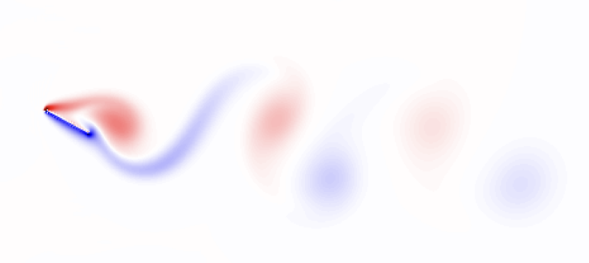
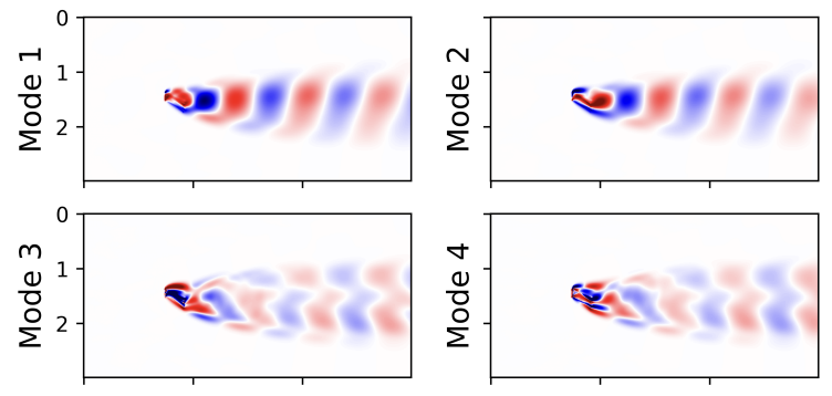
- Example from Song2025
- High-dimensional output ($>10^4$) - the entire quasi-periodic flow field with an airfoil in motion
- The flow field $\vg$ modeled as a MVGPR $\vg=\vV\vf$
- Columns of $\vV$ are modes;
- $\vf$ are UVGPR as modal coordinates, fewer than 10
- Special covariance function ($\cos$) in $\vf$ for periodic motion
- More discussion later in the Dimensionality Reduction module.
Multiple Fidelities
Suppose now we have both
- High-fidelity (HF) dataset - sparse, expensive but more accurate $$ \cD_{HF} = \{\vx_i^{HF},y_i^{HF}\}_{i=1}^M $$
- Low-fidelity (LF) dataset - abundant, cheap but less accurate $$ \cD_{LF} = \{\vx_i^{LF},y_i^{LF}\}_{i=1}^N $$
- Typically $M\ll N$.
We could construct multi-fidelity (MF) surrogate as follows
- First a LF surrogate with the relatively large LF dataset
- Then correct it using the sparse HF dataset. $$ \hat{y}_{MF}(\vx) = \rho \hat{y}_{LF}(\vx) + \hat{\delta}(\vx) $$ where $\rho$ is a multiplicative correction, and $\hat{\delta}$ is called the discrepancy function.
As a special case of MVGPR
- This is when $x_{LF}$ and $x_{HF}$ coincide
- Two independent UVGPRs for LF data $f_{LF}$ and discrepancy $f_{\delta}$
- Linearly combine the two to form a MVGPR $\vg$
$$ \vg = \begin{bmatrix} g_1 \\ g_2 \end{bmatrix} = \begin{bmatrix} 1 & 0 \\ \rho & 1 \end{bmatrix} \begin{bmatrix} f_{LF} \\ f_{\delta} \end{bmatrix} $$ where $g_2=f_{MF}$ is what we want.
- The matrix kernel function is
$$ \vK = \begin{bmatrix} 1 & 0 \\ \rho & 1 \end{bmatrix} \begin{bmatrix} k_{LF} & 0 \\ 0 & k_{\delta} \end{bmatrix} \begin{bmatrix} 1 & 0 \\ \rho & 1 \end{bmatrix}^\top = \begin{bmatrix} k_{LF} & \rho k_{LF} \\ \rho k_{LF} & \rho^2k_{LF} + k_{\delta} \end{bmatrix} $$
- Note the special triangular structure in the matrix; this is called an AR(1) approach, AR for auto-regressive.
Practical implementation:
- Fit a LF GP from LF dataset, $\hat{y}_{LF}$.
- Fit a MF GP from HF dataset, using $\hat{y}_{LF}$ as if a special mean function.
- (This procedure can keep going if >2 datasets are available).
Both steps only require a scalar GP fitting capability.
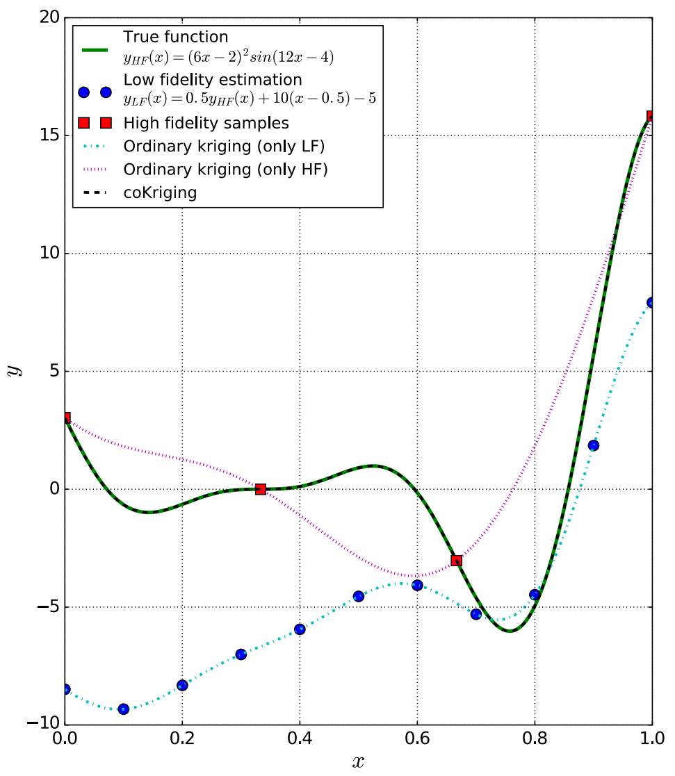
(example from Rokita2018)
Side note on "fidelity"
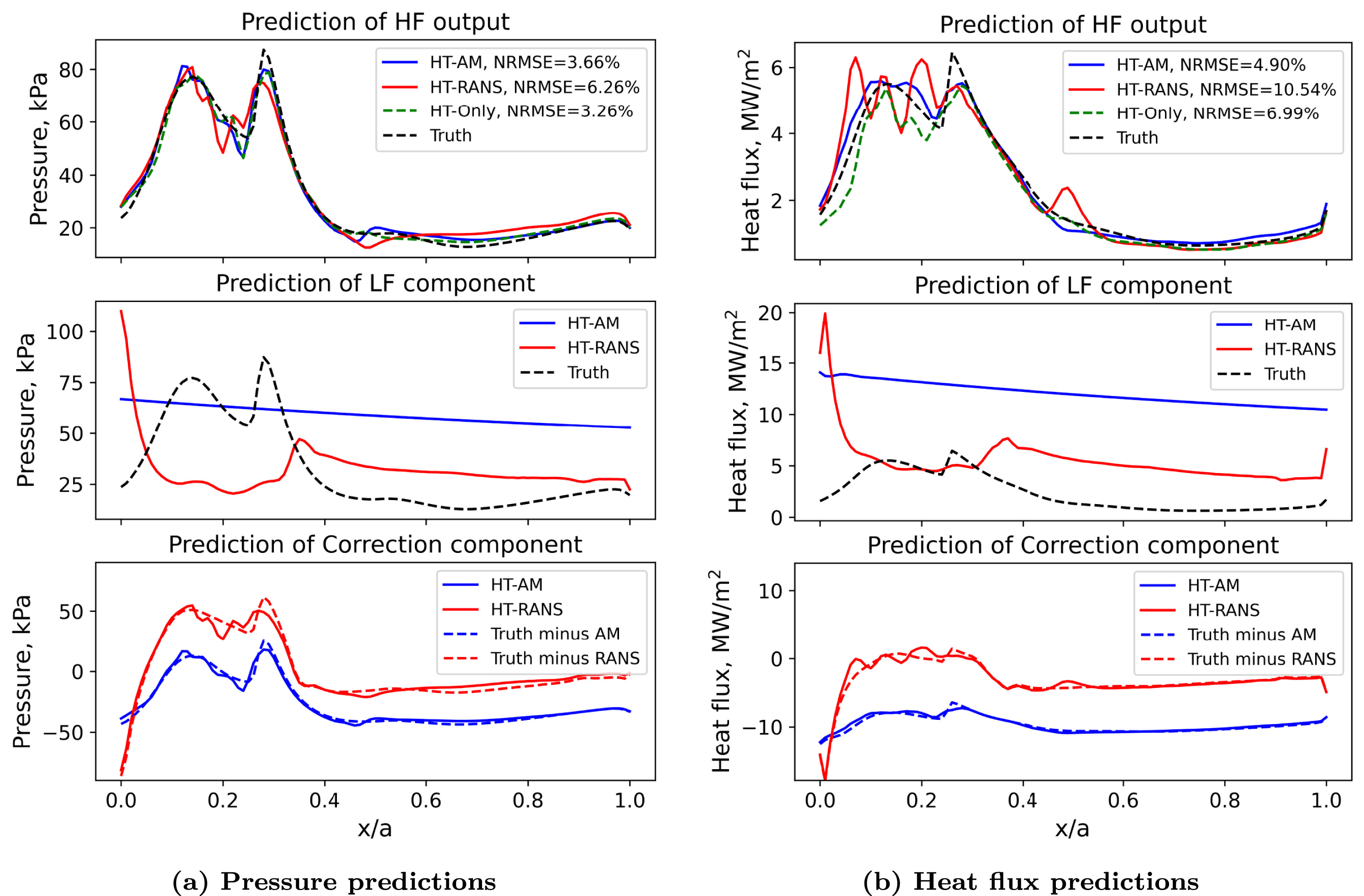
- In physics-based modeling, higher-fidelity means containing more physics
- In example, low-to-high: AM, RANS, HT
- In multi-fidelity surrogate modeling, higher-fidelity means higher correlation to truth
- In example, low-to-high: RANS, AM, HT
- Using wrong combination results in worse prediction!
- See example in Huang2022
Adding Gradients
Sometimes we have an augmented dataset where the gradients are available: $$ \cD=\left\{\left(\vx_i, y_i, \frac{\partial y_i}{\partial\vx}\right)\right\}_{i=1}^N $$
- This is possible, e.g., when using a differentiable solver, and perhaps becoming more common.
- Assuming $\vx\in\bR^d$ in the following. Possibly $d\gg 1$.
Brutal-force strategy I
Indirect: Still treat as regular GP, but augment dataset with possibly
- Fictitious points: Nearby actual sample points and predicted from the gradient. $$ \left(\vx_i, y_i, \frac{\partial y_i}{\partial\vx}\right) \Rightarrow \left(\vx_i, y_i+\frac{\partial y_i}{\partial\vx}\delta\vx_j\right),\quad j=1,2,\cdots,d $$
- Extra points: Nearby actual sample points and directly computed from the target function.
$$
\left(\vx_i, y_i, \frac{\partial y_i}{\partial\vx}\right) \Rightarrow \left(\vx_i, y(\vx_i+\delta\vx_j)\right),\quad j=1,2,\cdots,d
$$
- Technically this case does not even need the actual gradient.
- While easy to implement, but challenge - Severely enlarged dataset
- From $N$ to $(d+1)N$ points
- Costs $O((d+1)^3N^3)$ to train
- No guarantee to reproduce exact gradients
Example implementation of this strategy: SMT.
Brutal-force strategy II
Multiple UVGPR: Treat output and gradients as multiple (correlated) outputs $$ \left(\vx_i, y_i, \frac{\partial y_i}{\partial\vx}\right) \Rightarrow \left(\vx_i, \left[y_i,\frac{\partial y_i}{\partial\vx}\right]\right) $$
- Use the same covariance for each output, and fit $(d+1)$ times of UVGPR.
- Costs $O((d+1)N^3)$.
- Potential issue: No guarantee to reproduce exact gradients.
A better idea
Design matrix covariance function to account for gradient information.
Knowing the scalar UVGP: $$ f(\vx) \sim \GP(m(\vx),k(\vx,\vx')) $$ The GP and its gradient actually satisfy $$ \begin{bmatrix} f \\ \frac{\partial f}{\partial \vx} \end{bmatrix} \sim \GP\left( \begin{bmatrix} m \\ \frac{\partial m}{\partial \vx} \end{bmatrix}, \begin{bmatrix} k & \frac{\partial k}{\partial \vx'} \\ \frac{\partial k}{\partial \vx} & \frac{\partial^2 k}{\partial \vx\partial \vx'} \end{bmatrix} \right) $$
- Given only scalar $m$ and $k$, one can construct the matrix version
- Exactly reproduce the gradients (but however at the cost of $O((d+1)^3N^3)$)
More details: Laurent2017 and Dalbey2013.
1D example
- Function to fit: $y(x) = 10x^2 + \sin(4\pi x)$
- Consider $m(x)=0$ and SE kernel $k(x,y)=\exp(-(x-y)^2/l)$
- Devise matrix covariance by gradients $$ \vK(x,y) = \begin{bmatrix} k(x,y) & \frac{2}{l}(x-y)k(x,y) \\ -\frac{2}{l}(x-y)k(x,y) & \frac{2}{l} k(x,y) - \frac{4}{l^2} (x-y)^2k(x,y) \end{bmatrix} $$
- Compare with "naive" UVGPR with scalar SE for output + gradient.
f, ax = plt.subplots(ncols=2, figsize=(12,4))
for _i in range(2):
    ax[_i].plot(Xtrn, Ytrn[:,_i], 'rs', label='Data')
    ax[_i].plot(Xtst, Yscl[:,_i], 'b-', label='UVGPR')
    ax[_i].plot(Xtst, Ygrd[:,_i], 'k-', label='GPR w/ Grad')
    ax[_i].plot(Xtst, Ytst[:,_i], 'r--', label='Truth')
ax[0].legend(); ax[0].set_ylabel('y'); ax[1].set_ylabel('dy/dx'); ax[1].set_xlabel('x');

f = plt.figure()
plt.loglog(Ns, err[0], 'b-', label='UVGPR')
plt.loglog(Ns, err[1], 'k-', label='GPR w/ Grad')
plt.legend(); plt.xlabel('# samples'); plt.ylabel('Rel. Error');

(Another 2D example from [Dalbey2013])
Dynamical Systems
Lastly, we consider the application scenario of learning dynamical systems, either discrete-time or continuous-time $$ x_{n+1}=f(x_n),\quad\text{or}\quad \dot{x}=f(x) $$ assuming $x\in\bR^d$.
- In terms of GP, this is the multi-variate case.
- There are numerous way of applying GP to the dynamics. Below we illustrate just one example.
A 2D example
$$ \begin{bmatrix} \dot{x} \\ \dot{y} \end{bmatrix} = \begin{bmatrix} -f(\theta)y \\ f(\theta)x \end{bmatrix},\quad f(\theta) = 3/2 - \cos(\theta),\quad \theta=\tan^{-1}(y/x) $$
- We show below that the dynamics is actually on a circle.
- This is typical for systems with constraints (e.g., robotic arms) or inherent "symmetry" (e.g., rigid-body rotation)
f, ax = plt.subplots(ncols=2, figsize=(10,3))
ax[0].plot(tt, data_traj[:,0], 'b-'); ax[0].plot(tt, data_traj[:,1], 'r-')
ax[0].set_xlabel('t'); ax[0].set_ylabel('[x, y]');
ax[1].plot(*data_traj.T, 'b.')
for _i in range(0, Ntrain, 30):
    _x = data_traj[_i]; _y = _x + 0.4*fvec(_x).squeeze()
    ax[1].plot([_x[0], _y[0]], [_x[1], _y[1]], 'k-')
ax[1].set_xlabel('x'); ax[1].set_ylabel('y'); ax[1].set_aspect('equal', adjustable='box')

Next we try two models to learn the dynamics
- Assuming we know exactly $[\dot{x}, \dot{y}]$
- Model 1: "Naive" UVGPR that fits each dimension individually.
- Model 2: MVGPR with specialized covariance structure.
Note the following correlation in the dynamics $$ \begin{bmatrix} \dot{x} \\ \dot{y} \end{bmatrix} = \begin{bmatrix} -f(\theta)y \\ f(\theta)x \end{bmatrix} = \begin{bmatrix} -y \\ x \end{bmatrix}f(\theta) $$ This hints us to devise a special matrix covariance function $$ \vK(x,y,x',y') = \begin{bmatrix} -y \\ x \end{bmatrix}f(\theta)f(\theta') \begin{bmatrix} -y' & x' \end{bmatrix} = k(\theta,\theta') \begin{bmatrix} yy' & -yx' \\ -xy' & xx' \end{bmatrix} $$
f, ax = plt.subplots(ncols=2, figsize=(10,3))
for _i in range(2):
    ax[_i].plot(tt, sscl.y[_i], 'b-', label='UVGPR')
    ax[_i].plot(tt, stan.y[_i], 'k-', label='GP w/ tan')
    ax[_i].plot(tt, data_traj[:,_i], 'r--', label='Truth')
    ax[_i].set_xlabel('t')
ax[0].legend(); ax[0].set_ylabel('x'); ax[1].set_ylabel('y');

f = plt.figure()
plt.plot(tt, Yscl[:,0], 'b-', label='UVGPR') # Failed to capture xdot
plt.plot(tt, Ytan[:,0], 'k-', label='GP w/ tan')
plt.plot(tt, data_xdot[:,0], 'r--', label='Truth')
plt.legend(); plt.xlabel('t'); plt.ylabel('x_dot');

So far,
- We assumed the rates $[\dot{x}, \dot{y}]$ are known
- We assumed the tangent vectors (i.e., $[-y, x]$) are known
- The dynamics deviates from the circle after ~5 cycles
All these problems can be resolved - see Huang2025 for more details.