K-Means Clustering
- Previous lecture we talked about PCA
- To obtain a compressed representation of each data point with significantly fewer dimensions
- Alternatively we can use Clustering
- To compress the number of points, i.e., picking typical point(s) to represent a class of points.
Goal: Partition data $\X = \{ x_1, \dots, x_n \} \subset \R^d$ into $K$ disjoint clusters.
- Points within a cluster should be more similar to each other than to points in other clusters.
- Estimate cluster centers $\mu_k \in \R^d$ for $k=1,\dots,K$
- Estimate cluster assignments $z_j \in \{1,\dots,K\}$ for each point $x_j$
Usually, we fix $K$ beforehand, and need to use model selection to overcome this limitation.
Algorithm
First, pick random cluster centers $\mu_k$. Then, repeat until convergence:
E-Step: Assign $x_j$ to the nearest cluster center $\mu_k$, $$ z_j = \arg\min_k || x_j - \mu_k ||^2 $$
M-Step: Re-estimate cluster centers by averaging over assignments: $$ \mu_k = \frac{1}{\sum_{j=1}^N z_{jk}} \sum_{j=1}^N x_j z_{jk} $$ where $\sum_{j=1}^N z_{jk}=N_k$ the number of samples in cluster $k$.
We will explain the "E-step" and "M-step" later.
Mixture Models
Clustering problems motivate the definition of a mixture model.
- Observe data from multiple base distributions $p_k(x|\theta_k)$ over the same space.
- Proportion of each distribution given by mixing weights $\pi = (\pi_1,\dots,\pi_K)$
- Don't know which distribution each point comes from.
Mixture Models for Clustering
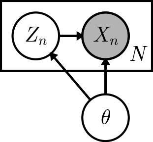
In clustering, we represent mixtures via latent cluster indicators, $$ \begin{align} z_n &\sim \Cat[\pi] & \forall\, n = 1,\dots,N \\ x_n \mid z_n &\sim p_{z_n}(\cdot \mid \theta_{z_n}) & \forall\, n = 1,\dots,N \end{align} $$ where
- $x_n$ is the observed variable, i.e. which cluster does the data point belong to.
- $z_n$ is the "latent" variable, as it is inferred during training and not observed.
- $\Cat[\pi]$ is a multi-class distribution for $z_n,\ n = 1,\dots,N$, such that
- $z_n\in \{0,1\}$
- $p(z_n=1)=\pi_n$, and $\sum_{n=1}^N=\pi_n$.
Gaussian Mixture Models
In a Gaussian Mixture Model, the base distributions are Gaussian.
- Cluster $k$ has mean $\mu_k$, covariance $\Sigma_k$
- These can be written as $$ \begin{align} p(z_n) &= \prod_{k=1}^K \pi_k^{z_{nk}} \\ p(x_n \mid z_n) &= \prod_{k=1}^K \mathcal{N}(x_n \mid \mu_k, \Sigma_k)^{z_{nk}} \end{align} $$ where $z_{nk}$ is the $k$th component of $z_n$, i.e. whether $x_n$ belongs to cluster $k$.
A Two-Cluster Example
Here are the contours of each base distribution plotted together:
plot_gmm()

Inference & Learning of GMM
Model: Specification $$ \begin{align} \theta &= (\vec\pi, \vec\mu, \vec\Sigma) && \text{model parameters} \\ z_n &\sim \Cat[\pi] && \text{cluster indicators} \\ x_n | z_n, \theta &\sim \mathcal{N}(\mu_{z_n}, \Sigma_{z_n}) && \text{base distribution} \end{align} $$
Goal: Since only the data points $x_n$ are observed, we wish to
- Learn the cluster parameters $\mu_{z_n}$, $\Sigma_{z_n}$
- Infer the cluster assignments $z_n$ for each point $x_n$
We will use the Expectation Maximization algorithm.
- Same general idea as K-means, but probabilistic
- Alternate between guessing latent variables and re-estimating parameters.
GMM: Complete Log Likelihood
The complete data log-likelihood for a single datapoint $(x_n, z_n)$ is $$ \begin{align} \log p(x_n, z_n | \theta) &= \log \prod_{k=1}^K \left[\pi_k \mathcal{N}(x_n \mid \mu_k, \Sigma_k)\right]^{z_{nk}} \\ &= \sum_{k=1}^K z_{nk} \log \left[\pi_k \mathcal{N}(x_n \mid \mu_k, \Sigma_k)\right] \end{align} $$
If we knew $z_{nk}$, then the MLE of $\pi_k$, $\mu_k$, and $\Sigma_k$ is trivial. (Hint: To find $\pi_k$, one needs to incorporate a constraint $\sum\pi_k=1$)
GMM: Hidden Posterior
And if we knew $\mu_k$ and $\Sigma_k$, but not $z_{nk}$, we can try to eliminate the latter.
The "hidden" posterior for $z_n$ of a single point can be found using Bayes' rule: $$ \begin{align} p(z_{nk} = 1 | x_n, \theta) &= \frac{p(x_n | z_{nk} = 1, \theta) p(z_{nk} = 1 | \theta)}{p(x_n | \theta)} \\ &= \frac{\pi_k \mathcal{N}(x_n | \mu_k, \Sigma_k)}{\sum_{k'=1}^K \pi_{k'} \mathcal{N}(x_n | \mu_{k'}, \Sigma_{k'})} \equiv r_{nk} \end{align} $$
The quantity $r_{nk}$ means the responsibility that cluster $k$ takes for datapoint $x_n$. And further, the expectation of $z_{nk}$ w.r.t. the posterior is, $$ E_z[z_{nk}]=r_{nk} $$
GMM: E-Step
The expected complete likelihood w.r.t. the hidden posterior is $$ \begin{align} E_z[ \log p(\X,Z|\theta)] &= \sum_{n=1}^N \sum_{k=1}^K E_z\big[ z_{nk} \big] \log \pi_k \mathcal{N}(x_n \mid \mu_k, \Sigma_k) \\ &= \sum_{n=1}^N \sum_{k=1}^K r_{nk} \log \pi_k + \sum_{n=1}^N \sum_{k=1}^K r_{nk} \log \mathcal{N}(x_n \mid \mu_k, \Sigma_k) \end{align} $$
Now the unknown $z_{nk}$ is gone! (But $r_{nk}$ depends on $z_{nk}$ though)
GMM: M-Step
During the M-Step, we optimize the lower bound with respect to $\theta=(\pi,\mu,\Sigma)$. The updates are $$ \begin{gather} \pi_k = \frac{1}{N} \sum_{n=1}^N r_{nk} = \frac{r_k}{N} \quad \mu_k = \frac{\sum_{n=1}^N r_{nk} x_n}{r_k} \\ \Sigma_k = \frac{\sum_{n=1}^N r_{nk} x_n x_n^T}{r_k} - \mu_k \mu_k^T \end{gather} $$
where $r_k = \sum_{n=1}^N r_{nk}$ is the effective sample size for cluster $k$.
Verify the update as an exercise.
Then an iterative procedure:
- Initialize $\theta^0=(\pi^0,\mu^0,\Sigma^0)$
- E-step (cluster reassignment): Find $r_{nk}$ using $\theta^{k-1}=(\pi^{k-1},\mu^{k-1},\Sigma^{k-1})$
- M-step (parameter update): Update $\theta^k=(\pi^k,\mu^k,\Sigma^k)$ using $r_{nk}$
Compare to the K-means algorithm - GMM is "fuzzier", right?
Comment: Discrimitive vs. Generative
The GMM is one of the fewer generative models covered in class. The previous models we have learnt are discriminative.
Suppose, we want $p(Y|X)$, $Y$ is output, $X$ is input. For regression models, $p(Y|X)$ is the predictive distribution from which one gets the prediction with error estimate.
- For Discrimitve model:
- Assume form of $p(Y|X)$ directly
- Determine parameters in $p(Y|X)$ from data set
- MLE of LR: We assumed $p(Y|X)$ is Gaussian, parameterized it by $w$, and found $w$ from data
- Similarly for MAP of RR. Be careful that Bayes' rule is applied to the parameter $w$, not the input $X$.
- For Generative model:
- Assume forms of $p(X|Y)$, $p(Y)$
- Determine parameters in $p(X|Y)$, $p(Y)$ from data set
- Use Bayes' rule to compute $p(Y|X)$
- In Bayes' rule, we implicitly compute $p(X,Y)$. For GMM that is the complete liklihood
- From $p(X,Y)$ we can generate new $x$ that is not from data.
Expectation Maximization
Uses material from [Neal & Hinton 1998], [Do 2008], and [MLAPP]
CAUTION: This part is a general discussion of the EM algorithm and not a core requirement of this course.
Parameter Estimation with Latent Variables
Question: How can we perform MLE/MAP in latent variable models?
Complete Data Log-Likelihood
Suppose we observe both $X$ and $Z$. The complete data log-likelihood is $$ \ell_c(\theta) = P(X,Z | \theta) = \sum_{n=1}^N \log p(x_n, z_n | \theta) $$
[MLAPP]: This likelihood function is convex when $p(x_n,z_n | \theta)$ is an exponential family distribution.
Observed Data Log-Likelihood
In reality, we only observe $\X=(x_1,\dots,x_n)$. The observed data log-likelihood is given by $$ \begin{align} \ell(\theta | \X) &= \log p(\X | \theta) = \sum_{k=1}^N \log p(x_k | \theta) \\ &= \sum_{k=1}^N \left[ \log \sum_{z_k} p(x_k, z_k | \theta) \right] \end{align} $$
[MLAPP]: This likelihood function is non-convex even assuming exponential family distributions. Multiple modes make inference (NP) hard!
Tackling a Non-Convex Likelihood
How can we optimize the observed likelihood $\ell(\theta|\X)$?
- Gradient-based methods? Tricky to enforce constraints (e.g. positive-definiteness)
We need a different approach...
Observation: In most models, MLE/MAP is easy with fully observed data. We will alternate between
- E-Step: Inferring the values of the latent variables.
- M-Step: Re-estimating the parameters, assuming we have complete data.
Note the similarity to K-Means!
Optimizing via Lower-Bounds
From a theoretical standpoint, we will alternate between
- Estimating a lower bound $\L(q,\theta)$ on $\log p(\X|\theta)$
- Maximizing this lower bound to obtain a new estimate of $\theta$
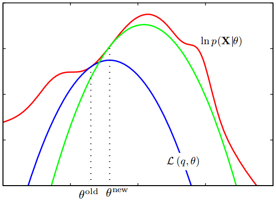 (Figure 9.14 of **[PRML]**)
Introducing Proxy Distribution
Our general approach will be to reason about the hidden variables through a proxy distribution $q(Z)$.
- Distribution $q$ is an approximation to $P(Z | \X, \theta)$
- We use $q$ to compute a lower bound on the log-likelihood.
The $q$ distribution will disappear later, but this perspective is useful for extending EM to new settings.
Review: Jensen's Inequality
For a convex function $f$, $$ \sum_{k=1}^K \lambda_k f(x_k) \geq f\left( \sum_{k=1}^K \lambda_k x_k \right) $$
If $\lambda_k \geq 0$ and $\sum_{k=1}^K \lambda_k = 1$.
Evidence Lower Bound - I
Through Jensen's inequality, we obtain the evidence lower bound (ELBO) on the log-likelihood: $$ \begin{align} \ell(\theta | \X) &= \log \sum_z p(\X, z | \theta) \\ &= \log \sum_z q(z) \frac{p(\X, z | \theta)}{q(z)} \\ &\geq \sum_z q(z) \log \frac{p(\X, z | \theta)}{q(z)} \equiv \L(q, \theta) \end{align} $$ Important: the choice of distribution $q(z)$ is arbitrary, above holds for all $q$.
Evidence Lower Bound - II
We can rewrite the lower bound $\L(q, \theta)$ as follows: $$ \begin{align} \ell(\theta | \X) \geq \L(q,\theta) &= \sum_z q(z) \log \frac{p(\X,z|\theta)}{q(z)} \\ &= \sum_q q(z) \log p(\X,z|\theta) - \sum_z q(z) \log q(z) \\ &= E_q[\log p(\X,Z|\theta)] - E_q[\log q(z)] \end{align} $$
Connection to Relative Entropy
Though not discussed in this course, it is possible to define the Kullback–Leibler divergence, or relative entropy, between two probabilitistic distributions $p$ and $q$, $$ \begin{align} D_{KL}(q || p) &= E_q[-\log p(Z)] + E_q[\log q(Z)] \\ &= H[q,p] - H[q] \geq 0 \end{align} $$ which quantifies the similarity between $p$ and $q$.
It is easy to show $\L(q,\theta)$ differs from a relative entropy by only a constant wrt $\theta$: $$ \begin{align*} D_{KL}(q || p(Z|\X,\theta)) &= H(q, p(Z|\X,\theta)) - H(q) \\ &= E_q[ -\log p(Z|\X,\theta) ] - H(q) \\ &= E_q[ -\log p(Z,\X | \theta) ] - E_q[ -\log p(\X|\theta) ] - H(q) \\ &= E_q[ -\log p(Z,\X | \theta) ] + \log p(\X|\theta) - H(q) \\ &= -\mathcal{L}(q,\theta) + \mathrm{const.} \end{align*} $$
In other words, we are essentialy trying to iteratively update the distribution $q$ to match the true unknown distribution $p$.
ELBO: Tightness
This yields a second proof of the ELBO, since $D_{KL} \geq 0$, $$ \boxed{ \log p(\X | \theta) = D_{KL}(q || p(Z | \X, \theta)) + \mathcal{L}(q,\theta) \geq \mathcal{L}(q,\theta) } $$
The quality of our bound $\L(q,\theta)$ depends heavily on the choice of proxy distribution $q(Z)$.
Remark: Maximizing $\L(q, \theta)$ with respect to $q$ is equivalent to minimizing the relative entropy between $q$ and the hidden posterior $P(Z|\X,\theta)$. Hence, the optimal $q$ is exactly the hidden posterior, for which $\log p(\X|\theta) = \L(q,\theta)$.
The bound is tight, i.e. we can make it touch the log-likelihood. Refer back to the PRML plot.
Idea of Expectation Maximization
Finding a global maximum of the likelihood is difficult in the presence of latent variables. $$ \hat\theta_{ML} = \arg\max_\theta \ell(\theta | \X) = \arg\max_\theta \log p(\X|\theta) $$
Instead, the Expectation Maximization algorithm gives an iterative procedure for finding a local maximum of the likelihood.
- Under the assumption that the hidden posterior $P(Z|\X,\theta)$ is tractable.
- Exploits the evidence lower bound $\ell(\theta|\X) \geq \L(q,\theta)$.
Consider only proxy distributions of the form $$ q_\vartheta(Z) = p(Z | \X, \vartheta) $$
- The optimal value for $\vartheta$, in the sense that $\L(\vartheta, \theta) \equiv \L(q_\vartheta, \theta)$ is maximum, depends on $\theta$.
- Similarly, the optimal $\theta$ depends on $\vartheta$.
- This suggests an iterative scheme.
Expectation Maximization: E-Step
Suppose we have an estimate $\theta_t$ of the parameters. To improve our estimate, we first compute a new lower bound on the observed log-likelihood, $$ \vartheta_{t+1} = \arg\max_\vartheta \L(\vartheta, \theta_t) = \theta_t $$
Since $q_\vartheta(Z) = p(Z|\X,\vartheta)$, we know from before that $\vartheta=\theta_t$ maximizes $\L(\vartheta, \theta)$.
Expectation Maximization: M-Step
Next, we estimate new parameters by optimizing over the lower bound. $$ \begin{align} \theta_{t+1} &= \arg\max_\theta \L(\vartheta_{t+1}, \theta) \\ &= \arg\max_\theta E_q[\log p(\X,Z|\theta)] - E_q[\log q_\vartheta(z)] \\ &= \arg\max_\theta E_q[ \log p(\X,Z | \theta) ] \end{align} $$
The last line optimizes over the expected complete data log-likelihood.
Expectation Maximization: Algorithm
Expectation maximization performs coordinate ascent on $\L(\vartheta,\theta)$.
Expectation Maximization: Convergence
Theorem: After a single iteration of Expectation Maximization, the observed data likelihood of the parameters has not decreased, that is, $$ \ell(\theta_t | \X) \leq \ell(\theta_{t+1} | \X) $$
Proof: This result is a simple consequence of all our hard work so far! $$ \begin{align} \ell(\theta_t | \X) &= \mathcal{L}(q_{\vartheta_{t+1}}, \theta_t) & \text{(Tightness)} \\ &\leq \mathcal{L}(q_{\vartheta_{t+1}}, \theta_{t+1}) & \text{(M-Step)} \\ &\leq \ell(\theta_{t+1} | \X) & \text{(ELBO)} \end{align} $$
Expectation Maximization: Convergence
Theorem: (Neal & Hinton 1998, Thm. 2) Every local maximum of $\L(q, \theta)$ is a local maximum of $\ell(\theta | \X)$.
General Advice for EM
- Specify the model. Identify the observed variables, hidden variables, and parameters. Draw a graphical model.
- Identify relevant probabilities. This includes the complete data likelihood $p(X,Z|\theta)$ and hidden posterior $p(Z|X,\theta)$.
- Derive the E-Step. Compute $E_q[\log p(\X,Z|\theta)]$.
- Derive the M-Step. Take derivatives and set to zero, when possible. Otherwise, gradient-based methods can be used.