$$ \newcommand{\R}{\mathbb{R}} \renewcommand{\vec}[1]{\mathbf{#1}} \newcommand{\X}{\mathcal{X}} \newcommand{\D}{\mathcal{D}} $$
Dimensionality Reduction
High-dimensional data may have low-dimensional structure.
- We only need two dimensions to describe a rotated plane in 3d!
- We have seem a few examples in the previous lecture
plot_plane()

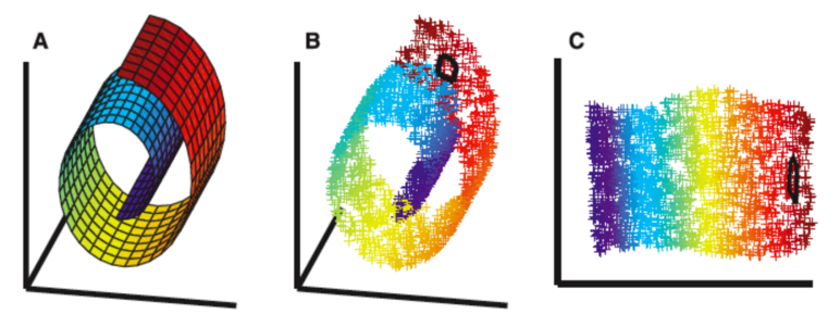
Data may even be embedded in a low-dimensional nonlinear manifold.
- How can we recover a low-dimensional representation?
In physics, a seemingly high-dimensional problem, e.g. an unsteady flow field, might live in a low-dimensional subspace.
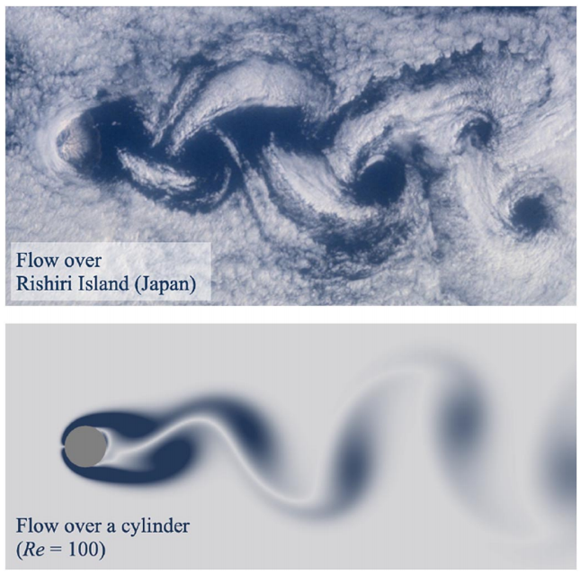
An interesting paper on modal analysis of fluid flow.
Principal Components Analysis
Given a set $X = \{x_n\}$ of observations
- in a space of dimension $D$,
- find a linear subspace of dimension $M < D$
- that captures most of its variability.
There are perhaps 10+ ways to understand PCA, and perhaps 10+ names, e.g.
- Proper Orthogonal Decomposition (POD), from the fluid dynamics community
- Karhunen-Loeve Expansion (KLE), from the statistics/probability community
we will start with the classical deterministic approach
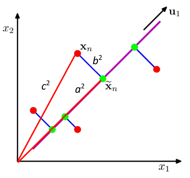
PCA: Equivalent Descriptions
- maximizing the variance of the projection, or
- minimizing the squared approximation error.
With mean at the origin $ c_i^2 = a_i^2 + b_i^2 $, with constant $c_i^2$
- Minimizing $b_i^2$ maximizes $a_i^2$ and vice versa
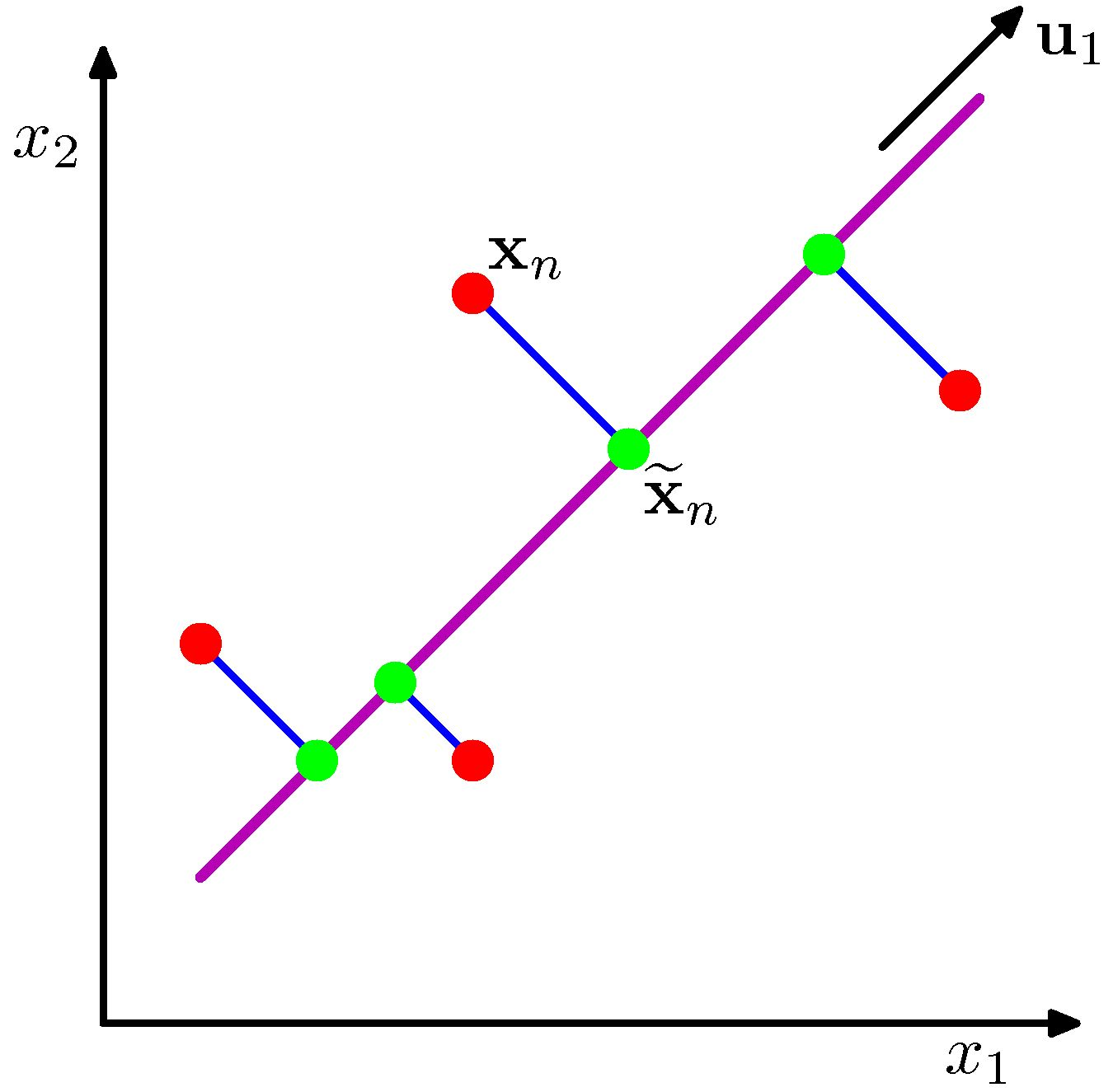
PCA: The First Principal Component
Given data points $\{x_n\}$ in $D$-dim space, define
Mean $\bar x = \frac{1}{N} \sum_{n=1}^{N} x_n $
Data covariance ($D \times D$ matrix):
$$ S = \frac{1}{N} \sum_{n=1}^{N}(x_n - \bar x)(x_n - \bar x)^T$$
Let $u_1$ be the principal component we want.
- Unit length $u_1^T u_1 = 1$
- Projection of $x_n$ is $u_1^T x_n$
Goal: Maximize the projection variance over directions $u_1$: $$ \frac{1}{N} \sum_{n=1}^{N}\{u_1^Tx_n - u_1^T \bar x \}^2 = u_1^TSu_1$$
Use a Lagrange multiplier to enforce $u_1^T u_1 = 1$
- Maximize: $u_1^T S u_1 + \lambda(1-u_1^T u_1)$
Derivative is zero when $ Su_1 = \lambda u_1$
- That is, $u_1^T S u_1 = \lambda $
So $u_1$ is eigenvector of $S$ with largest eigenvalue.
PCA: The Next PC's
Repeating the above procedure, one obtains the "less" principal components.
New Goal: Maximize the projection variance over directions $u_k$: $$ u_k^TSu_k$$
With two constraints now:
- Normalization: $u_k^Tu_k=1$
- Orthogonality to previous PC's: $u_k^T u_i = 0$, for $i=1,2,\cdots,k-1$
Ultimately, $u_k$ is the $k$th eigenvector of $S$, with eigenvalue $\lambda_k$.
You will dive into the details in the homework.
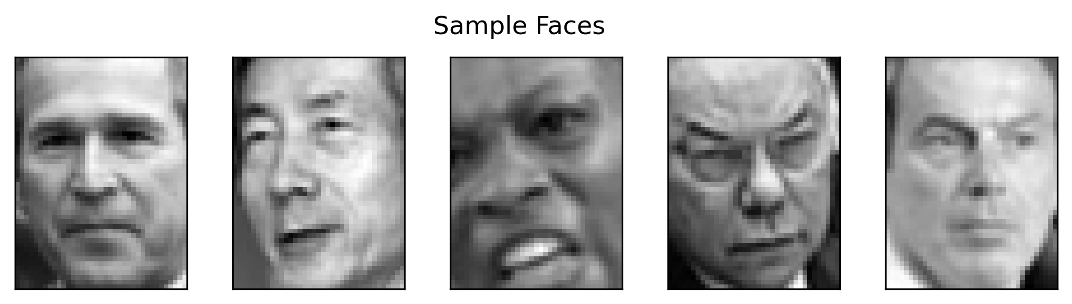
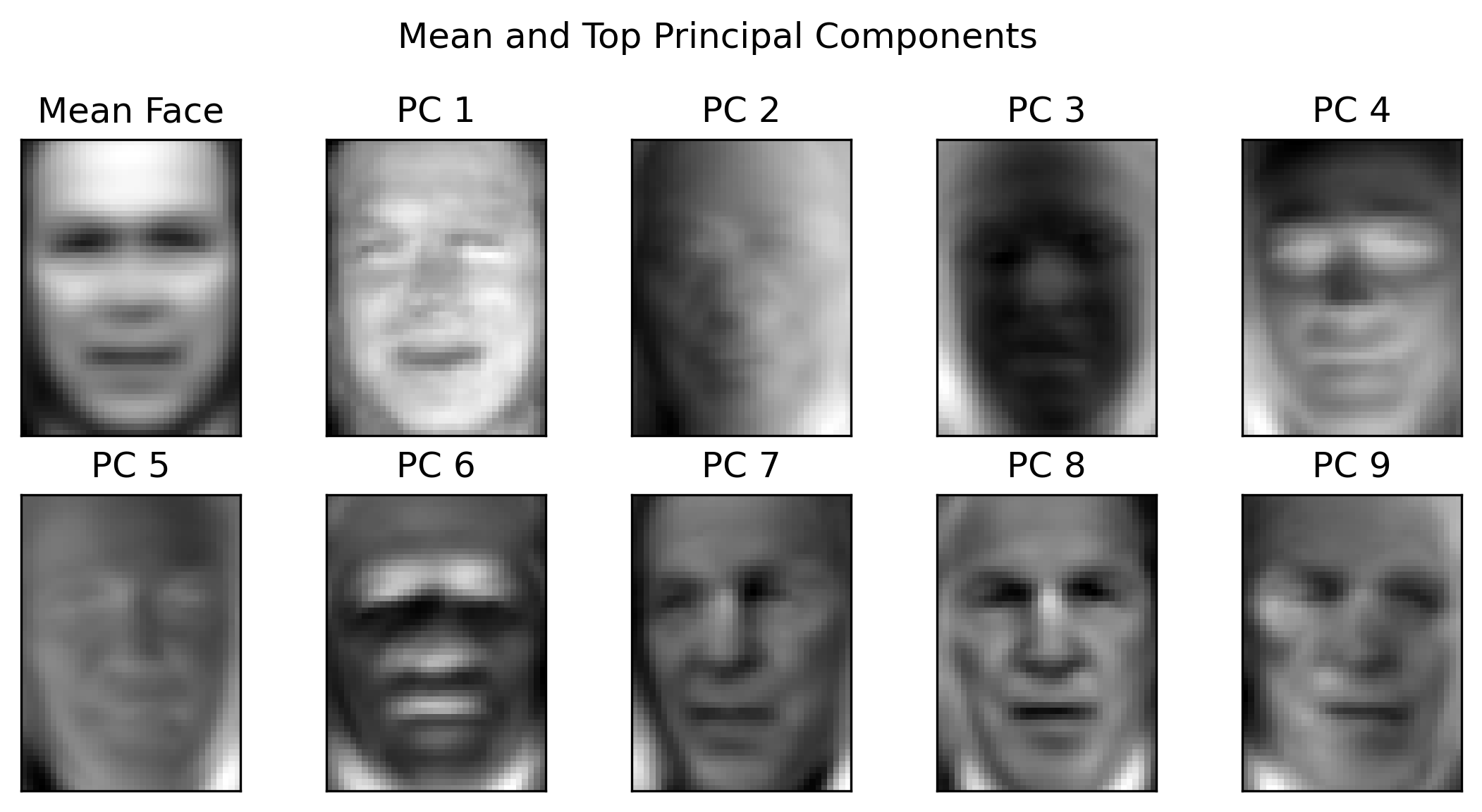
Example - Eigenfaces 1/2
- $1560$ images of faces
- Image size: $50 \times 37$ - $1850$ pixels per image
- Reshape as a vector in $\mathbb{R}^{1850}$
Reconstruction from PCA
One major application of PCA is to approximate the original $D$-dim data by $M$-dim coordinates, $D\gg M$,
$$ x \approx \bar{x} + c_1u_1 + c_2u_2 + \cdots + c_Mu_M \equiv \bar{x} + Uc $$
where $U\in\mathbb{R}^{D\times M}$ and $c\in\mathbb{R}^M$.
To find $c$, note that $U^TU=I$, because of orthogonality
$$ c = U^T(x-\bar{x}) $$
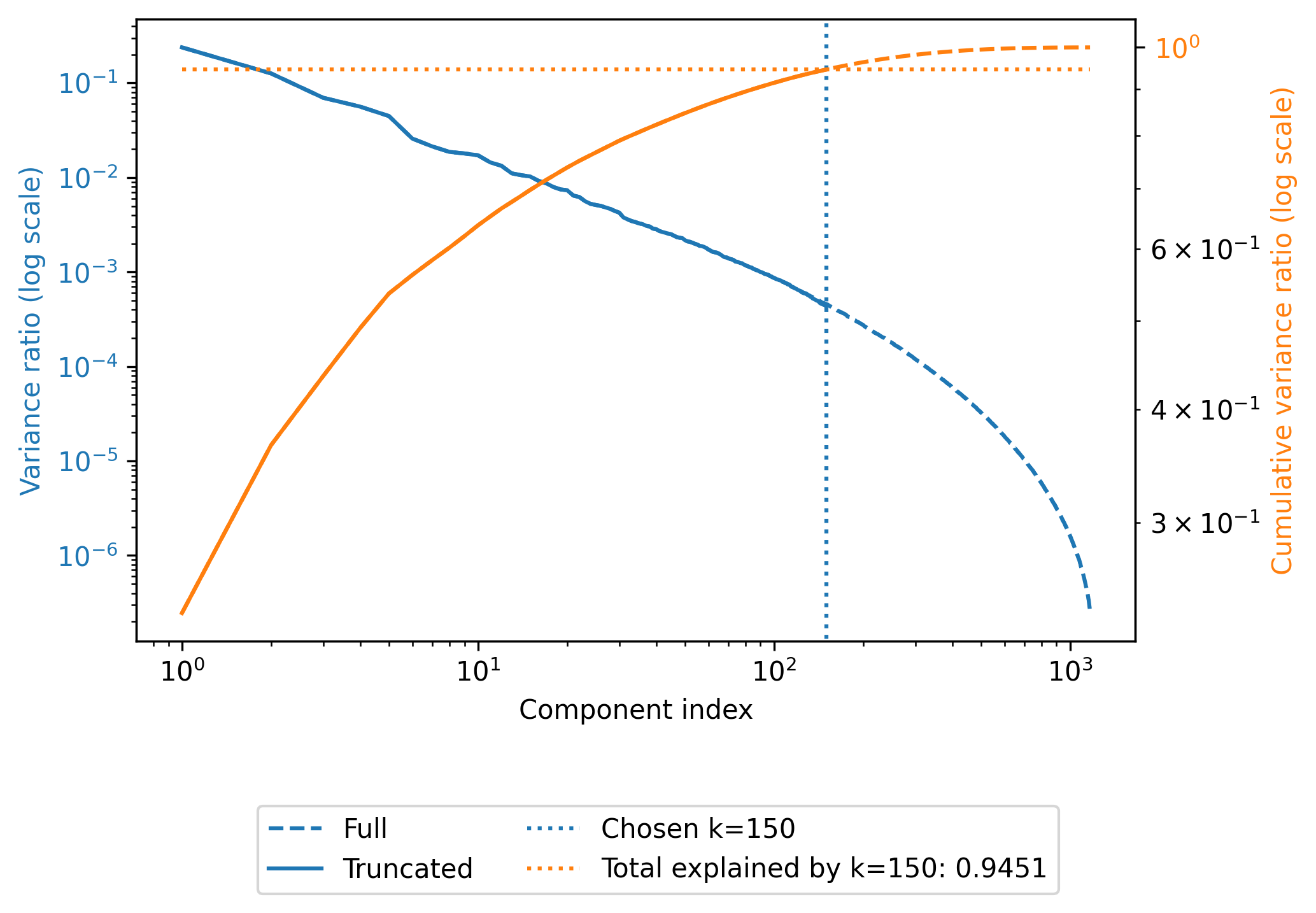
Explained variances
- Each $u_i$ has a variance $\sigma_i^2$ - Spread of data along $u_i$.
- The chosen $M$ PC's: Explained variances in PCA - $\sigma_1^2$, $\sigma_2^2$, $\cdots$, $\sigma_M^2$.
- Explained variance ratio $$ r = \frac{\sum_{i=1}^M\sigma_i^2}{\sum_{i=1}^D\sigma_i^2} $$
- If $r\approx 1$, all data is explained using the $M$ components (instead of all the $D$ dimensions).
- In practice one chooses $r$ to determine $M$.
Advantages
- Storage: Instead of storing the full $N\times D$ numbers, store
- PC coordinates: $c$'s, size $N\times M$ (again $D\gg M$)
- PC's (Overhead): $D\times (M+1)$
- Overall $O(M(D+N))$
- Every new data: Add $M$, instead of $D$.
- Modeling, e.g., linear regression:
- Instead of learning weights in $\mathbb{R}^D$
- Learn weights in $\mathbb{R}^M$
- Much fewer to learn, and maybe more stable and robust
- Data analysis: Understanding dominant patterns in data - can reveal physics
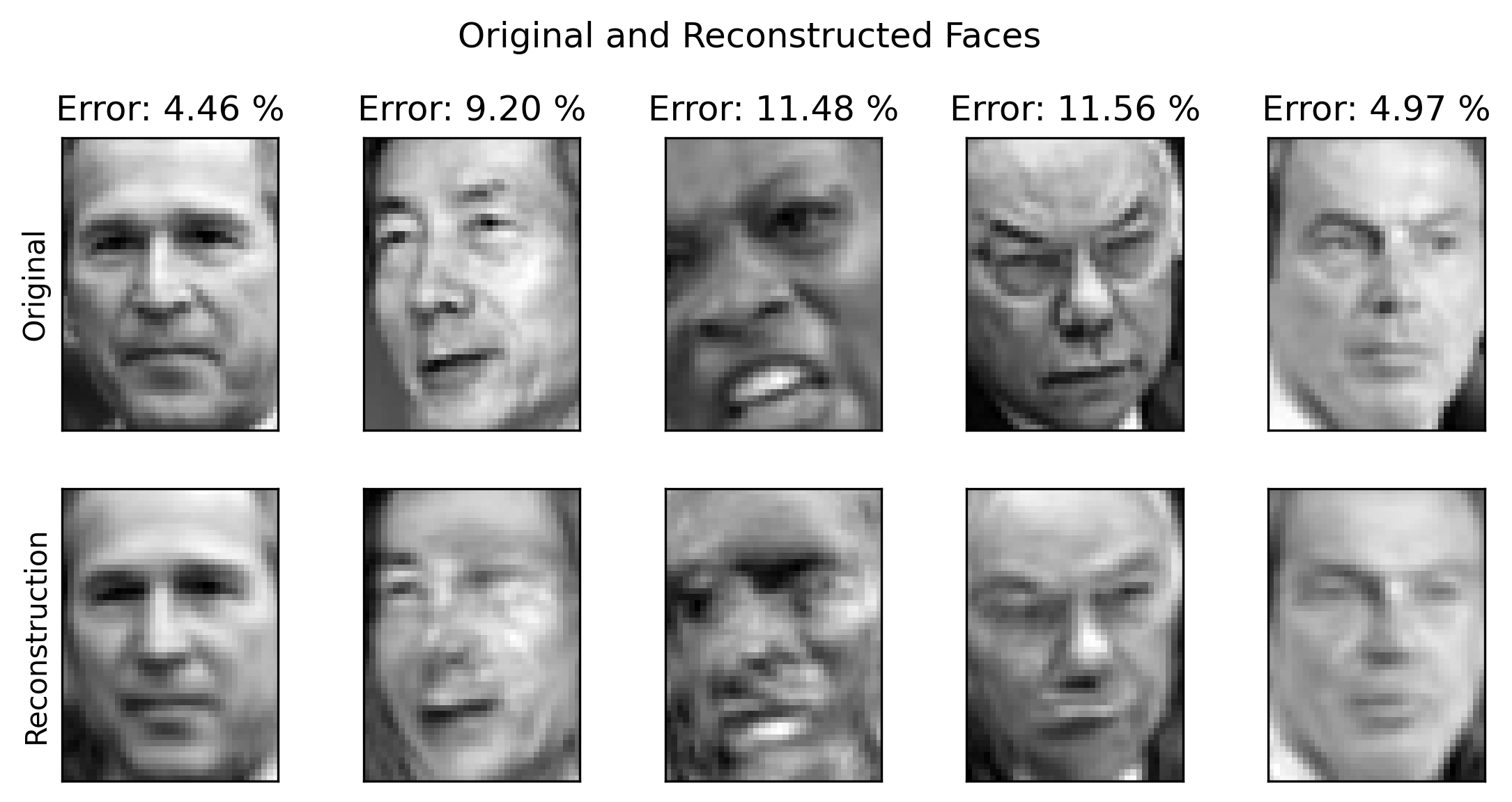
Example - Eigenfaces 2/2
- Choosing $M=150$ for $N=1560$ and $D=1850$.
- Compression ratio $$ \approx \frac{ND}{M(D+N)} = \frac{1560\times 1850}{150\times(1560 + 1850)} \approx 5.64 $$
Note trade-off in accuracy.
PCA and SVD
The search of the principal components of the data ends up in solving an eigenvalue problem (EVP) associated with the empirical covariance matrix $$ S u_i=\lambda_i u_i $$
- One would want to choose the largest $M$ eigenvalues and the associated eigenvectors.
- These eigenpairs maximizes the variances $\sigma_i^2 = u_i^T S u_i$, and minimizes the projection error $J=\sum_{M+1}^D\lambda_i$.
- Another way to look at explained variance ratio - for a small number, e.g. $\epsilon=0.01$, $$ \frac{\sum_{i=1}^M\lambda_i}{\sum_{i=1}^D\lambda_i} = 1-\frac{J}{\sum_{i=1}^D\lambda_i} \geq 1-\epsilon $$
Now consider data matrix $X\in\mathbb{R}^{N\times D}$, whose rows are the data vectors, mean subtracted.
- Suppose now $D\gg N$, so it is inefficient to do an EVP for $S=\frac{1}{N}X^TX$, which has a cost of $O(D^3)$.
- Instead, one could do the following EVP at reduced cost $O(N^3)$, $$ \frac{1}{N}XX^T (X u_i)=\lambda_i (X u_i)\quad\Rightarrow\quad \tilde{S} v_i=\lambda_i v_i $$
- The eigenvalues are the same as those associated with $u_i$.
- And to recover $u_i$ from $v_i$, $$ u_i=\frac{1}{\sqrt{N\lambda_i}}X^T v_i $$
Furthermore, consider the singular value decomposition of the data matrix $$ X=U\Sigma V^T,\quad X^TX=V\Sigma^2 V^T,\quad XX^T=U\Sigma^2U^T $$
- $u_i$ and $v_i$ are the left and right singular vectors of $X$, and $\lambda_i=\sigma_i^2$.
- Alternatively, one could do the SVD of $X$ to find the principal components of the dataset.
- While full SVD is expensive, there is a randomized SVD algorithm that can find max components efficiently.
- The SVD approach also called the snapshot method
Side note - 1
A theoretical guarantee, Eckart–Young theorem
For a centered matrix $X\in\mathbb{R}^{n\times m}$, say $n>m$, if we want a rank-$r$ approximation $Y$ to $X$, i.e., $$ \min_{\operatorname{rank}(Y)=r} \|X - Y\|_F $$ Then using the SVD of $X=U\Sigma V^\top$, and its rank-$r$ truncation $$ Y = U_r \Sigma_r V_r^\top, $$ and the approximation error is $$ \|X - Y\|_F = \sqrt{\sum_{i=r+1}^m \sigma_i^2} $$
Thus, SVD provides the optimal low-rank approximation in Frobenius norm.
Side note - 2
It is also possible to hard-threshold the SVD truncation. For an $m\times n$ matrix, let $m$ be the median of SV's, one can truncate all the SV's below $\omega(\beta)m$, where $$ \beta=m/n,\quad \omega(\beta) \approx 0.56\beta^3 - 0.95\beta^2 + 1.82\beta + 1.43 $$ But I would always recommend looking at the data and the spectrum of SV's before truncating.
Ref: M. Gavish and D. Donoho, The Optimal Hard Threshold for Singular Values is $4/\sqrt{3}$, arXiv 1305.5870.
Probabilistic PCA
We can view PCA as solving a probabilistic latent variable problem. $$ \begin{align*} x &= Wz + \mu + \epsilon \\ z &\sim \mathcal{N}(0, I_M) \end{align*} $$ where we describe
- data $x \in \R^D$ in terms of
- latent variable $z \in \R^M$ in lower dimensional space, via
- linear transformation $W \in \R^{D \times M}$ that maps $z \mapsto x$
- and $\epsilon$ is a D-dimensional zero-mean Gaussian-distributed noise variable with covariance $\sigma^2 I$.
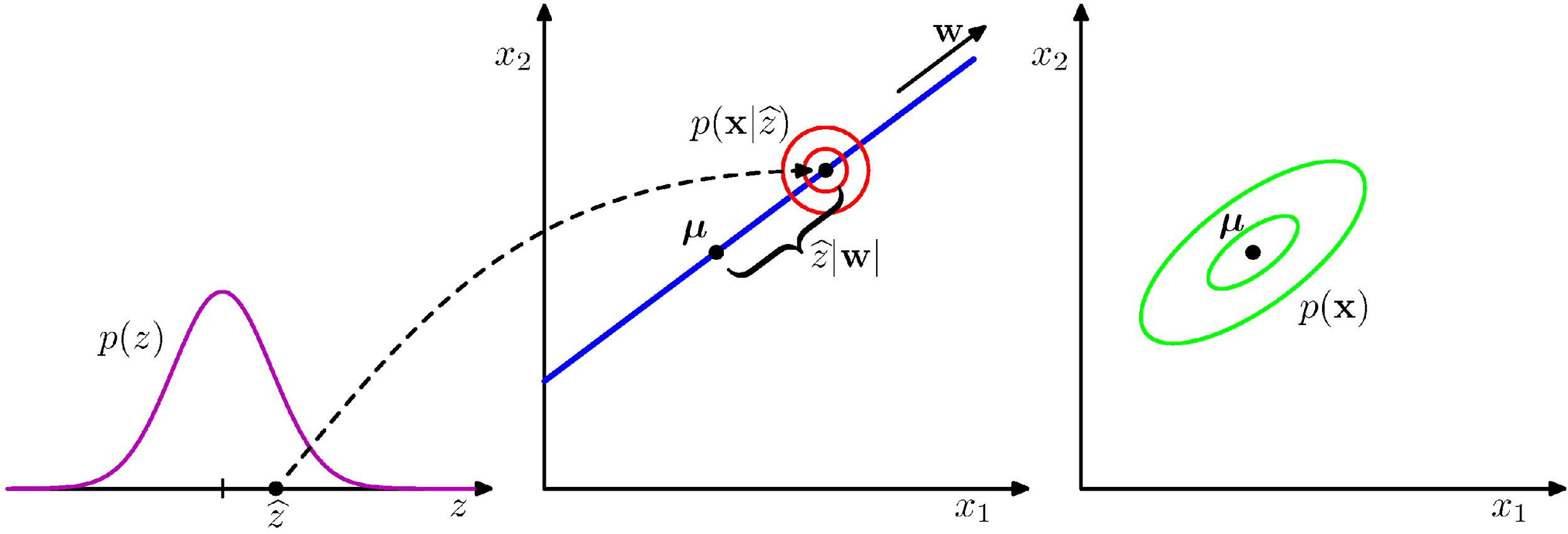
Given the model $p(x|z)$, we can infer
$$ \mathbb{E}[x] = \mathbb{E}[Wz + \mu + \epsilon] = \mu $$
$$ \begin{align*} \text{Cov}[x] &= \mathbb{E}[(Wz + \epsilon)(Wz + \epsilon)^T] \\ &= \mathbb{E}[Wzz^TW^T] + \mathbb{E}[ \epsilon \epsilon^T] \\ &= WW^T + \sigma^2 I \end{align*} $$
Maximum Likelihood
$$ \begin{align*} &\quad \log p(X|\mu, W, \sigma^2) = \sum_n \log p(x_n| W, \mu, \sigma^2) \\ &\qquad = -\frac{ND}{2} \log 2\pi - \frac{N}{2} \log |C| -\frac{1}{2} \sum_n (x_n - \mu)^TC^{-1}(x_n - \mu) \\ C &= WW^T + \sigma^2 I \end{align*} $$
We can simply maximize this likelihood function with respect to $\mu, W, \sigma$.
- Mean: $\mu = \bar x$
- Noise (i.e., the "unexplained" variances): $$ \sigma_{ML}^2 = \frac{1}{D-M} \sum_{i=M+1} ^{D} \lambda_i $$
- Transform: $$W_{ML} = U_M (L_M - \sigma^2 I)^{\frac{1}{2}} R $$
The truncated dimensions manifest as uniform "noise", and
- $L_M$ is diag with the $M$ largest eigenvalues; so noise is due to the discarded eigenvalues/components in the data.
- $U_M$ is the $M$ corresponding eigenvectors, i.e. the PC's in standard PCA.
- $R$ is an arbitrary $M\times M$ rotation (i.e., $z$ can be defined by rotating “back”), note for any such $R$, one can define $\tilde{W}=WR$, and $\tilde{W}\tilde{W}^T=WRR^TW^T=WW^T$. So there is redundancy in $W$!
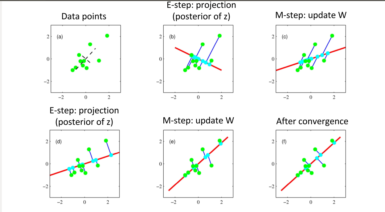
Probabilistic PCA: Other Formulations (Skip in class)
It is also possible to formulate the PCA using
- Expectation Maximization
- Bayesian approach
See [PRML] Chap. 12 for more details.
e.g., Expectation Maximization
which alternatively optimizes the $W$ and $z$ in the probabilistic formulation.
PCA with Regularization
Now that we are talking about SVD, the PCA can be also thought as an optimization problem, $$ U,W = \mathrm{argmax}\ \|X-UW\|_F^2 $$ such that $U\in\R^{D\times M}$ and $W\in\R^{M\times N}$; F-norm is the sqrt of sum of squares of all elements.
And it turns out SVD of $X$ gives the solution to the above optimization problem, as before.
But in terms of optimization we could do more: for example, sparse PCA by applying some regularization terms (recall from the regression methods).
A quadratic form is $$ U,W = \mathrm{argmax}\ \|X-UW\|_F^2 + \gamma \|U\|_F^2 + \gamma \|W\|_F^2 $$ which tries to minimize the magnitudes of the weights
- Or replace the F-norm with 1-norm for $W$, then we are asking to use as few modes as possible to describe the original data.
- More details in Ref: M. Udell, Generalized Low Rank Models
Sparse PCA may capture "multi-scale" behaviors in data
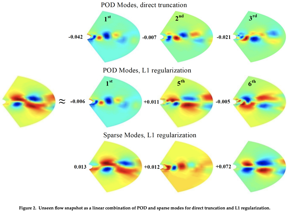
Ref: R. Deshmukh, etc., Basis Identification for Reduced Order Modeling of Unsteady Flows Using Sparse Coding
PCA with Missing Data
For another example, PCA of a dataset where some data in some dimensions are missing. The technique called Gappy POD can be used by constructing another optimization problem $$ U,W = \mathrm{argmax}\ ||P(X-UW)||_F^2 $$ where $P$ is a "mask" matrix with 0s and 1s specifying where the data is known.
In this 2D airfoil example, the method reconstructs the mode with 30% data missing.
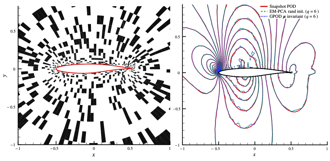
Ref: K. Lee, Unifying Perspective for Gappy Proper Orthogonal Decomposition and Probabilistic Principal Component Analysis
Karhunen-Loeve Expansion (skip in class)
One can also think a high-dimensional data point as a realization of a stochastic process - let's just look at a zero-mean Gaussian process, $y\sim GP(0,k(s,t))$.
Guaranteed by the so-called Mercer's theorem, the kernel can be expanded as $$ k(s,t) = \sum_{i=1}^\infty \lambda_i u_i(s)u_i(t) $$ where one needs to solve an integral eigenvalue problem (IEP) $$ \int k(s,t)u_i(s) ds = \lambda_i u_i(t) $$
Then the GP can be approximated as $$ y \approx \sum_{i=1}^M c_i \sqrt{\lambda_i} u_i(t) $$ where $c_i$ is a unit Gaussian variable.
In other words, the infinite-dimensional GP can be approximated using finitely $M$ properly chosen random variables.
In the practical sense, for example,
- Recall that if one obtains $N$ realizations of a zero-mean GP on a $[0,1]$ with 1000-point grid, one gets N 1000-dimension vectors $\{y_1,y_2,\cdots,y_N\}$.
- One can estimate the covariance matrix from the data $S=\frac{1}{N}\sum_{i=1}^N y_i y_i^T$
- $S$ is essentially the discrete version of $k(s,t)$
- And the eigenvalue decomposition of $S$ corrsponds to the IEP
- But as we have seen $S$ also produces the principal components
- In this context the following three are equivalent
- Eigenvectors of $S$
- Principal components of data
- Eigenfunctions of the stochastic process underlying the data
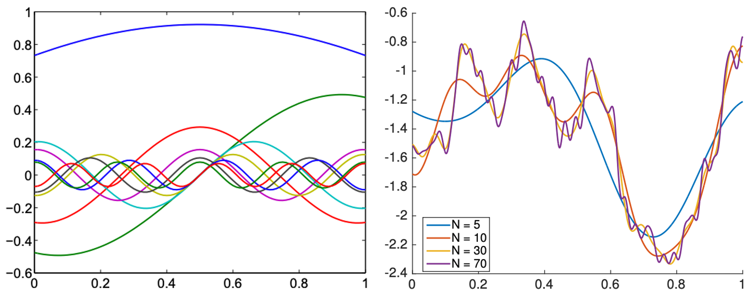
KLE of a GP with kernel $k(s,t)=\exp(-|s-t|)$ on domain $[0,1]$. The eigenfunctions are actually sinusoidal functions (left) and the GP is reconstructed well using >30 functions (right) - regardless of how many grid points are used in $[0,1]$
Ref: A. Alexanderian, A brief note on the Karhunen-Loeve expansion, arXiv 1509.07526.
Much more details: L. Wang, Karhunen-Loeve Expansions and their Applications, Ph.D. thesis, LSE.
Extending to Manifold Learning
There are many more dimension reduction algorithms, which are nonlinear, classified under the name "manifold learning". Due to the limit of time, these algorithms cannot be covered in class. However, the manifold module from the sklearn package is a good source for an introduction to (at least) the following algorithms,
- Isometric Mapping (Isomap)
- Locally Linear Embedding (LLE)
- Multidimensional scaling (MDS)
- t-distributed Stochastic Neighbor Embedding (t-SNE)
There is also methods from a somewhat different world, such as the Topological Data Analysis, for extracting nonlinear geometry from data.
Example: Kernel PCA
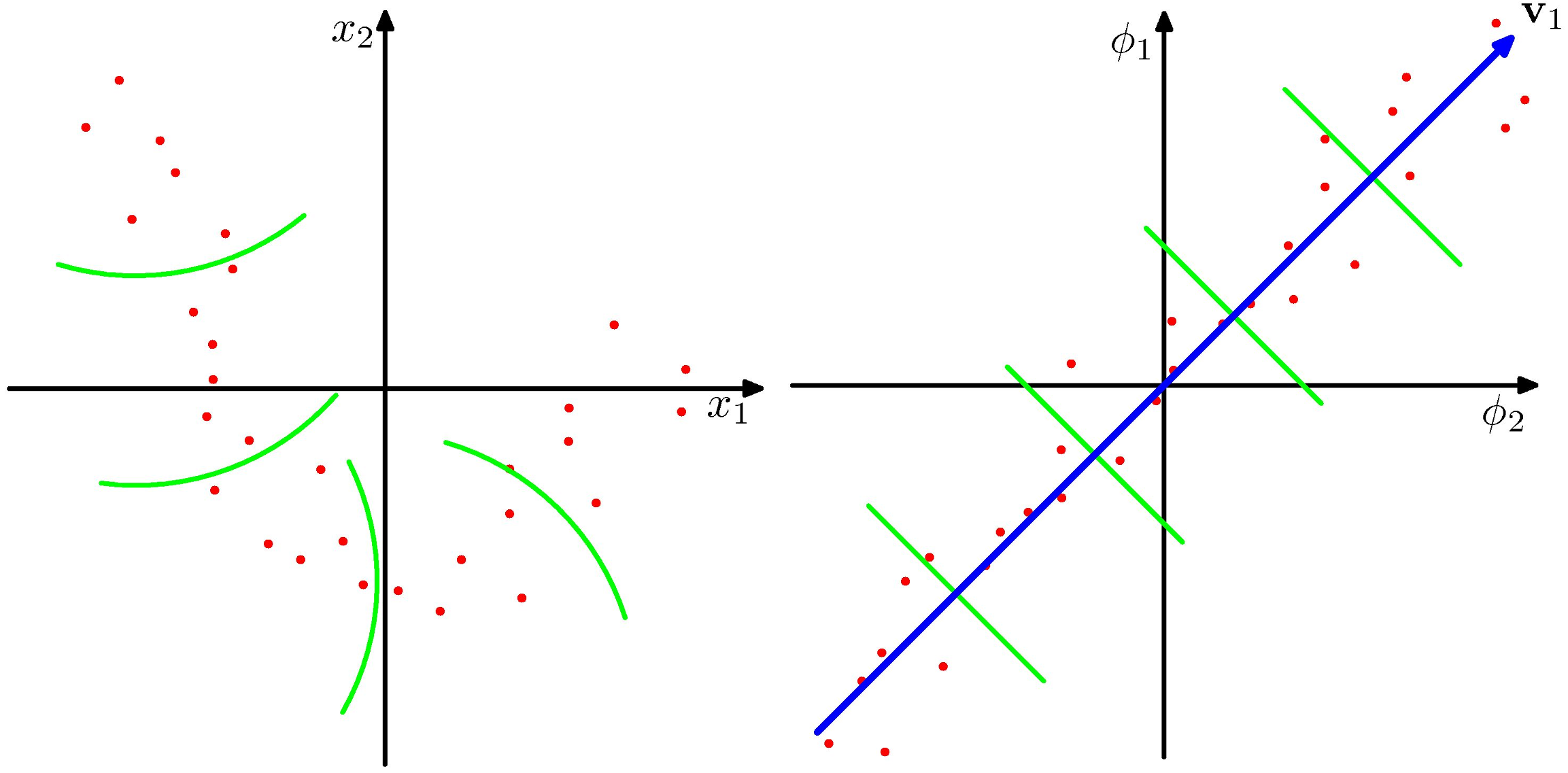
- Suppose the regularity that allows dimensionality reduction is non-linear. Left: nonlinear space; Right: "straightened" linear space.
- As with regression and classification, we can transform the raw input data $x_n$ to a set of feature values
$$ x_n \rightarrow \phi(x_n) $$
- Linear PCA (on the nonlinear feature space) gives us a linear subspace in the feature value space, corresponding to nonlinear structure in the data space.
Define a kernel, to avoid having to evaluate the feature vectors explicitly. $$ \kappa (x, x') = \phi(x)^T \phi(x') $$
And recall that the kernel defines another type of distance (now think in terms of variance maximization) $$ ||\phi(x) - \phi(z) ||^2 = \kappa(x,x) - 2\kappa(x,z) + \kappa(z,z) $$
Define the Gram matrix K of pairwise similarities among the data points: $$ K_{nm} = \phi (x_n)^T \phi(x_m) = \kappa (x_n, x_m) $$
Express PCA in terms of the kernel,
- Some care is required to centralize the data. $$ N\lambda x=Kx $$ As if working with $S$!
Tensor Train Decomposition
Extension to high-dimensional case
Motivation
For 2D data, we work with matrices, say $X\in\mathbb{R}^{n\times m}$.
- Full storage: $O(nm)$
- Rank-$r$ approximation: $O(nr+mr)$
But what about N-dimensional data, or tensors, $$ \mathcal{X} \in \mathbb{R}^{n_1 \times n_2 \times \dots \times n_d} $$
Examples
- Images over time (e.g., videos)
- Parametric PDE solutions
- Multi-way feature maps
- High-order polynomial expansions
Storage Explosion
Full storage requires $ \prod_{k=1}^d n_k. $
For example, if $n_k = 20$, $d=10$ then $20^{10} \sim 10^{13}$.
- Even moderate dimension leads to exponential growth!
One possibility is to reshape tensor into a matrix and apply SVD.
Say reshaping into $20^5 \times 20^5$, then truncate to rank $r$.
- It is still about $6\times 10^6$!
Problems:
- Matrix size becomes exponential in $d$
- Destroys multi-dimensional structure
- Computationally infeasible
We need low-rank tensor representations that scale linearly in dimension.
Definitions
For a tensor, $\mathcal{X}\in\mathbb{R}^{n_1 \times n_2 \times \dots \times n_d}$, denote its element at index $(i_1,\dots,i_d)$ as $$ \mathcal{X}(i_1,\dots,i_d). $$
Think it as a Numpy/Torch multi-dim array.
A tensor is in Tensor Train (TT) form if it can be written as
$$ \mathcal{X}(i_1,\dots,i_d) = G_1(i_1) G_2(i_2) \cdots G_d(i_d) $$
where $ G_k(i_k) \in \mathbb{R}^{r_{k-1} \times r_k} $, each core $ G_k \in \mathbb{R}^{r_{k-1} \times n_k \times r_k}, $
and $ r_k $ are TT-ranks, and $ r_0 = r_d = 1 $.
In other words, each index $i_k$ selects a matrix $G_k(i_k)$, and the tensor value is obtained by multiplying $d$ matrices.
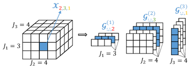
[From ResearchGate]
Storage problem solved
For simplicity, assume $n_k=n$ and $r_k=r$ for $k=1,2,\cdots,d$.
- Full storage: $O(n^d)$
- TT representation: $O(dnr^2)$
TT scales linearly in dimension $d$ as we hope!
But how do we compute TT decomposition?
Computing TT Decomposition
TT-SVD algorithm constructs the Tensor Train using sequential SVDs.
We factor the tensor dimension-by-dimension. At each step,
- Reshape into a matrix
- Compute truncated SVD
- Extract a TT core
- Pass the remainder to the next step
Step 1
Reshape: $$ X^{(1)} = \text{reshape}(\mathcal{X})\in \mathbb{R}^{n_1 \times (n_2 \cdots n_d)} $$
Compute truncated SVD up to rank $r_1$: $$ X^{(1)}\approx U_1 \Sigma_1 V_1^\top \equiv \hat{X}^{(1)} $$
Define: $$ G_1 = \text{reshape}(U_1) \in \mathbb{R}^{1 \times n_1 \times r_1} $$
Pass forward the remainder: $$ \bar{X}^{(2)} = \Sigma_1 V_1^\top \in \mathbb{R}^{r_1 \times (n_2 \cdots n_d)} $$
Step k
Reshape remaining tensor: $$ X^{(k)} = \text{reshape}(\bar{X}^{(k)}) \in \mathbb{R}^{(r_{k-1} n_k) \times (n_{k+1} \cdots n_d)} $$
Compute SVD: $$ X^{(k)} \approx U_k \Sigma_k V_k^\top \equiv \hat{X}^{(k)} $$
Define:
$$ G_k= \text{reshape}(U_k) \in \mathbb{R}^{r_{k-1} \times n_k \times r_k} $$
Pass forward remainder, and continue until (k=d).
Approximation Error
Let the singular values of $X^{(k)}$ be $$ \sigma^{(k)}_1 \ge \sigma^{(k)}_2 \ge \cdots $$
The tail energy discarded at step $k$ $$ \delta_k^2 = \|X^{(k)} - \hat{X}^{(k)}\|_F^2 = \sum_{j>r_k}\big(\sigma_j^{(k)}\big)^2 $$
Due to orthogonality of each step (proof not shown), the total error is $$ \|\mathcal X-\widehat{\mathcal X}\|_F^2 = \sum_{k=1}^{d-1}\delta_k^2 $$
Example
Consider a synthetic grayscale video of a small ball translating across a 2D grid.
Let the video be a tensor, $H=W=T=64$ $$ \mathcal{X} \in \mathbb{R}^{H \times W \times T} $$
Baseline (matrix SVD): flatten space and do SVD on
$$
X \in \mathbb{R}^{(HW)\times T}
$$
Truncation to rank $r$ yields storage $r(HW+T)$.
TT approach: Not only keeping $H \times W \times T$, but also granulating more $$ \tilde{\mathcal{X}} \in \mathbb{R}^{8\times 8 \times 8\times 8 \times 8 \times 8} $$ with storage $\sum_k r_{k-1} n_k r_k$.
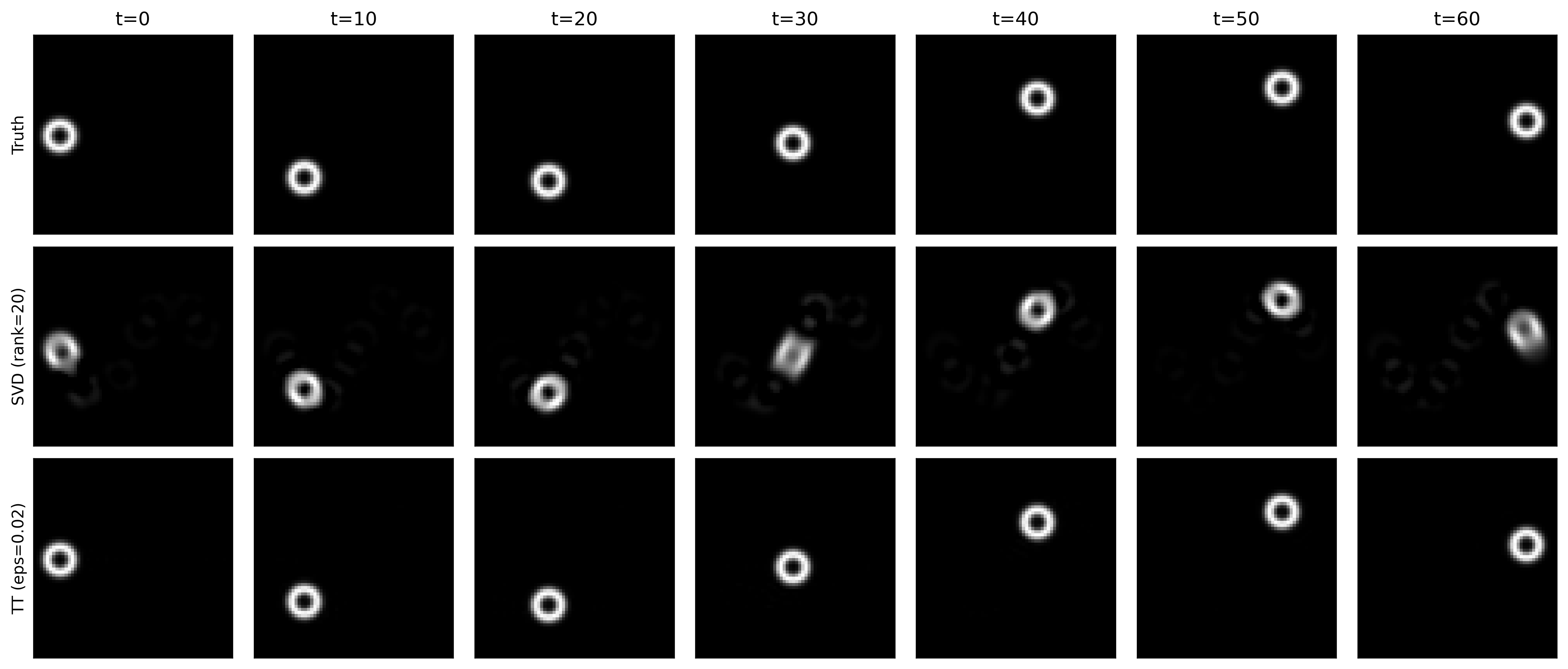
Reconstruction comparison - note the smearing circle in SVD
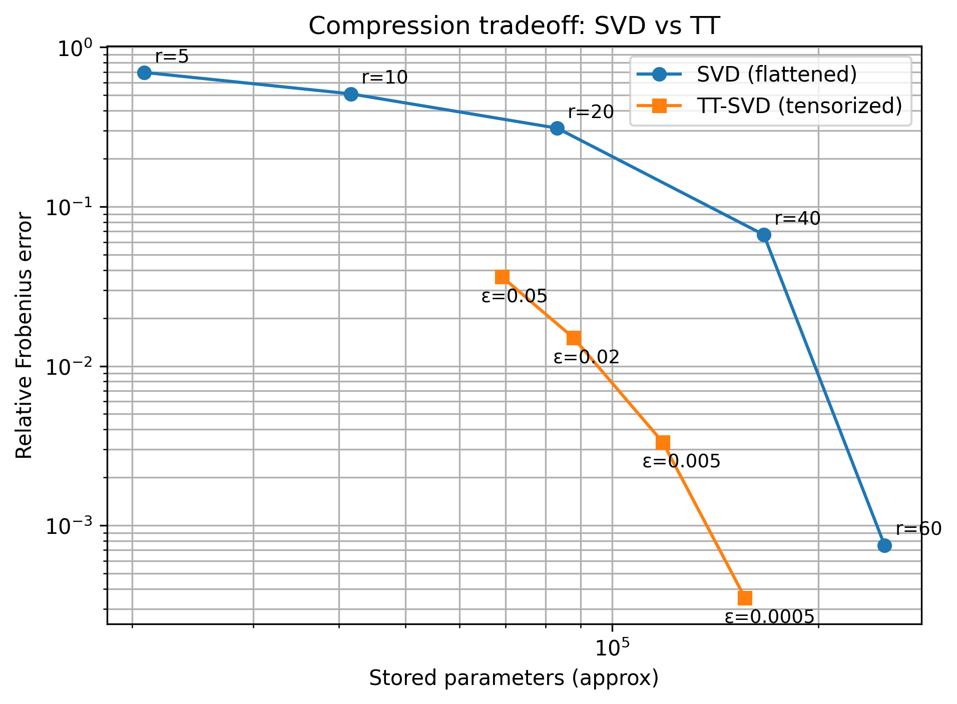
TT achieves fewer parameters with higher accuracy!
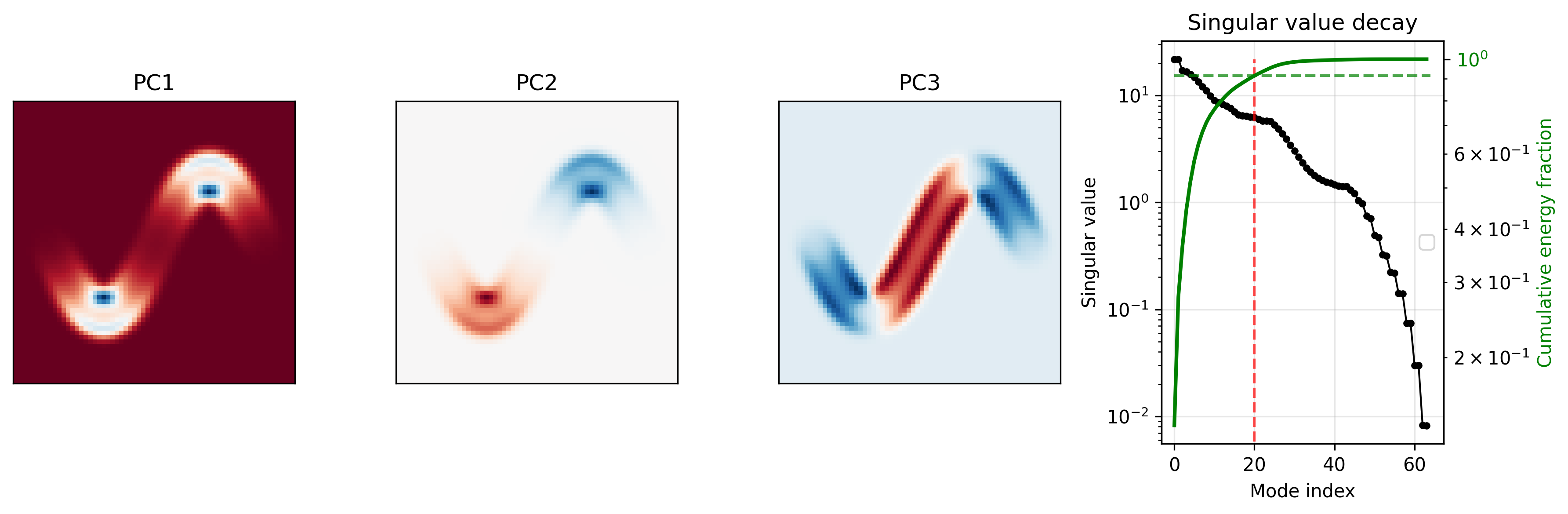
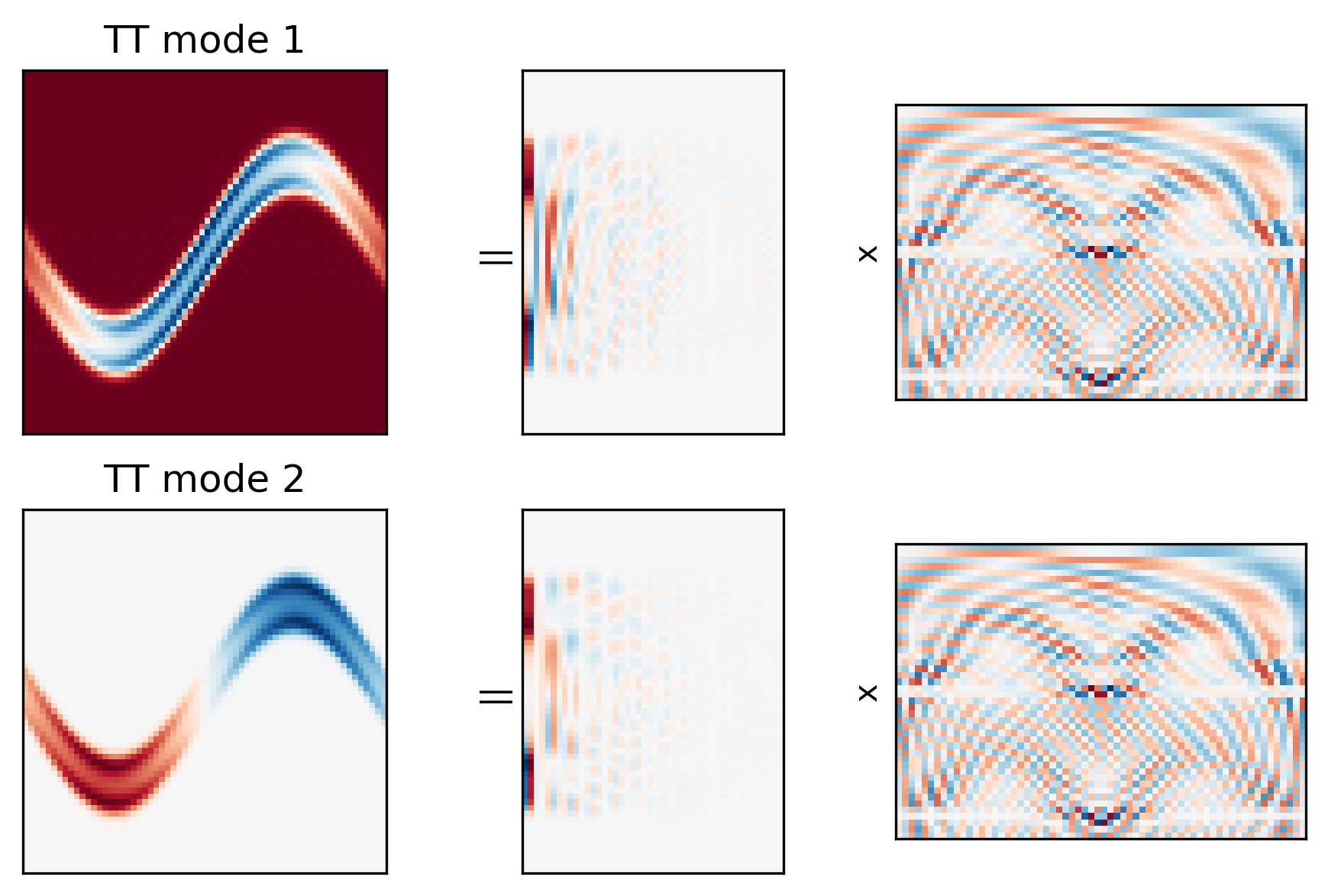
Under the hood - TT modes
More non-trivial to visualize. Take a simpler case of TT directly on $\mathcal{X}\in\mathbb{R}^{64\times64\times64}$ $$ \mathcal{X} = \underbrace{G_1}_{1\times H\times r_1}\quad\underbrace{G_2}_{r_1\times W \times r_2}\quad\underbrace{G_3}_{r_2\times T\times 1} $$
Consider "spatial" modes - $r_2$ modes of shape $H\times W$ - analogy of PC modes $$ \underbrace{M}_{H\times W \times r_2} = \underbrace{G_1}_{1\times H\times r_1}\quad\underbrace{G_2}_{r_1\times W \times r_2} $$
$G_3$ behaves like PC coordinates over time.
Show the first 2 spatial modes, and the corresponding factors from $G_1$ and $G_2$.
- Similar to SVD modes
- But improved compression via additional reduction in spatial modes.
Independent Components Analysis (Skip in class)
Uses material from [MLAPP] and [PRML]
Independent Component Analysis
Suppose N independent signals are mixed, and sensed by N independent sensors.
- Cocktail party with speakers and microphones.
- EEG with brain wave sources and sensors.
Can we reconstruct the original signals, given the mixed data from the sensors?
Independent Component Analysis
The sourcess must be independent.
- And they must be non-Gaussian.
- If Gaussian, then there is no way to find unique independent components.
Linear mixing to get the sensor signals x.
$x = As$ or $s = Wx$ (i.e., $W = A^{-1}$ )
$A$ are the bases, $W$ are the filters
ICA: Algorithm
There are several formulations of ICA:
- Maximum likelihood
- Maximizing non-Gaussianity (popular)
Common steps of ICA (e.g., FastICA):
- Apply PCA whitening (aka sphering) to the data
- Find orthogonal unit vectors along which the that non-Gaussianity are maximized $$ \underset{W}{\max}\hspace{1em} f(W \tilde x) \hspace{2em} s.t.\hspace{1em} WW^T = I$$ where f(x) can be "kurtosis", L1 norm, etc.
ICA: Step 1, Preprocessing
We use PCA Whitening to preprocess the data:
- Apply PCA: $ \Sigma = U \Lambda U^T $
- Project (rotate) to the principal components
- “Scale” each axis so that the transformed data has identity as covariance.
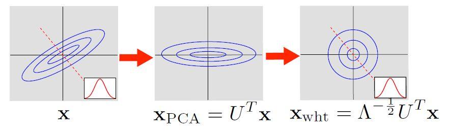
ICA: Step 2, Maximize Non-Gaussianity
Rotate to maximize non-Gaussianity
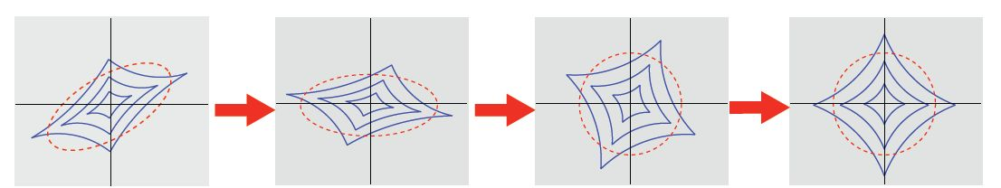
$$ \begin{align} x_{PCA} &= U^Tx = \Lambda^{-\frac{1}{2}} U^Tx \\ x_{ICA} &= V \Lambda^{-\frac{1}{2}} U^Tx \end{align} $$
ICA vs PCA
plot_ica_pca()

ICA: Mixture Example
Input Signals and Density
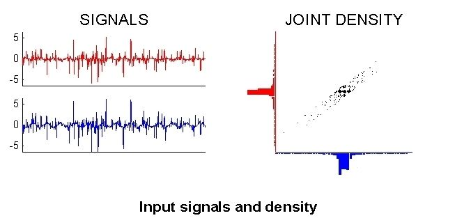
ICA: Mixture Example
To whiten the input data:
We want a linear transformation $ y = V x $
So the components are uncorrelated: $\mathbb{E}[yy^T] = I $
Given the original covariance $ C = \mathbb{E}[xx^T]$
We can use $V = C^{-\frac {1}{2}} $
Because $ \mathbb{E}[yy^T] = \mathbb{E}[Vxx^TV^T] = C^{-\frac {1}{2}} C C^{-\frac {1}{2}} = I $
ICA: Mixture Example
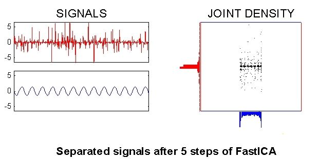
ICA: Summary
- Learning can be done by PCA whitening followed kurtosis maximization.
- ICA is widely used for blind-source separation
- The ICA components can be used for features.
- Limitation: difficult to learn overcomplete bases due to the orthogonality constraint