$$ \newcommand{\bR}{\mathbb{R}} \newcommand{\vf}{\mathbf{f}} \newcommand{\vg}{\mathbf{g}} \newcommand{\vv}{\mathbf{v}} \newcommand{\vw}{\mathbf{w}} \newcommand{\vx}{\mathbf{x}} \newcommand{\vy}{\mathbf{y}} \newcommand{\vA}{\mathbf{A}} \newcommand{\vB}{\mathbf{B}} \newcommand{\vU}{\mathbf{U}} \newcommand{\vV}{\mathbf{V}} \newcommand{\vW}{\mathbf{W}} \newcommand{\vX}{\mathbf{X}} \newcommand{\vtf}{\boldsymbol{\phi}} \newcommand{\vty}{\boldsymbol{\psi}} \newcommand{\vtF}{\boldsymbol{\Phi}} \newcommand{\vtS}{\boldsymbol{\Sigma}} \newcommand{\vtL}{\boldsymbol{\Lambda}} \newcommand{\cF}{\mathcal{F}} \newcommand{\cK}{\mathcal{K}} $$
TODAY: High-Dimensional System - III
- Issues of spatial decomposition
- Dynamic mode decomposition
References:
- [DMSC] Chap. 7
- http://dmdbook.com/
- [PyDMD] Documentation
Motivation
We first consider a general non-linear dynamical system, which is representative of many engineering problems:
$$ \dot{\vx} = \vf(\vx,t,\mu),\quad \vx(0)=\vx_0 $$
with (discrete-time) measurements:
$$ \vy_k=\vg(\vx_k) $$
Why interested in the dynamics:
- System diagnostics: feature extraction and interpretation
- Future state prediction
- Discovery of non-linear dynamics
- Modeling for control applications
We first consider a simple spatially-1D example consisting of
- A low-frequency decaying mode $\omega=-0.05+1.3i$
- A high-frequency growing mode $\omega=0.03+2.8i$
- White noise of constant uniform strength
titles = ['$f_1(x,t)$', '$f_2(x,t)$', '$f$']
data = [X1, X2, X]
_=pltContours(xgrid, tgrid, data, titles)

Question:
Is it possible to ...
- Extract the modes from the response?
- Recover the frequency of these modes?
- Predict the future responses?
First let's try PCA.
titles = ['Data', 'PCA Reconstruction', 'Residual']
data = [X, X_pca, X-X_pca]
_=pltContours(xgrid, tgrid, data, titles)

_=pltMD(mod_pca, dyn_pca.T, 'PCA') # Non-exact modes, non-exact periods

Issues with PCA:
- The reconstruction of the original dataset is close to perfect
- However, the modes are mixed up. As a result, the time response of each mode is noisy and contains multiple frequencies.
- Root of the problem: PCA does not account for the order information in data.
Dynamic Mode Decomposition to the rescue.
Dynamic Mode Decomposition
Review: Linear System
In DMD, we approximate the non-linear dynamical system by a low dimensional linear system: $$ \dot{\vx}=\bar{\vA}\vx $$ where $\bar{\vA}$ has eigenvalues $\bar{\lambda}=\zeta+\omega i$ and eigenvectors $\vtf$.
Then the solution is determined from the initial condition $\vx(0)=\vx_0$, $$ \vx=\sum_{i=1}^n b_i \vtf_i e^{\bar{\lambda}_i t} $$ where $b_i=\vtf_i^T\vx_0$
But typically the state measurement occurs at discrete time $\vx_j=\vx(t_j)$, with a time step size $\Delta t$, so one has a discrete linear system, $$ \vx_{k+1} = \vA \vx_k $$ where $\vA=\exp(\vA\Delta t)$, and $\vA$ has the same eigenvectors $\vtf$ as $\bar{\vA}$, but the eigenvalues become, $$ \lambda = \exp(\bar{\lambda}\Delta t),\quad \mathrm{or},\quad \bar{\lambda} = \frac{\log|\lambda|}{\Delta t} + \frac{\mathrm{Arg}(\lambda)}{\Delta t} i $$ And the solution given $\vx(0)=\vx_0$ is now written as, $$ \vx_{k+1}=\sum_{i=1}^n b_i \lambda_i^{k+1} \vtf_i $$
Review: Linear Stability
The eigenvalues determine the stability of the modes, i.e. whether the response decays or grows in time. Specifically, for the continuous case, we check $\zeta=Re(\bar{\lambda})$; for the discrete case, we check $|\lambda|$:
- $\zeta<0$, or $|\lambda|<1$: Decaying response, hence stable.
- $\zeta=0$, or $|\lambda|=1$: Neutrally stable.
- $\zeta>0$, or $|\lambda|>1$: Growing response, hence unstable.

Be careful with the boundaries - what happens when
- $q=0$: $\lambda_1=p$ and $\lambda_2=0$
- One direction is "unresponsive"
- $\Delta=0$: $\lambda_{1,2}=p/2$
- Two identical eigenvalues - do we always get two different eigenvectors?
We shall explore more later in nonmodal analysis (if time permits)
Setting up the Temporal decomposition
Now assume full-state measurement: $\vx_j=\vx(t_j)$
Assemble $m$ measurements into the following:
$$ \begin{align*} \vX &= [\vx_1 | \vx_2 | \cdots | \vx_{m-1}] \\ \vX^1 &= [\vx_2 | \vx_3 | \cdots | \vx_m] \end{align*} $$
If the system is linear, there is a discrete-time system matrix satisfying $$ \vX^1 = \vA\vX $$
This is a least squares problem, and the solution is $$ \vA = \vX^1 \vX^+ $$ where $\vX^+$ is the pseudo-inverse.
Again, be careful this $\vA$ is different from the $\bar{\vA}$ in the continuous system.
Algorithm
To find $\vA$, and the associated modes and eigenvalues, we carry out the following steps:
Step 1: Rank-r truncation $$ \vX=\vU_r\vtS_r\vV_r^* $$
Step 2: System matrix $$ \vA = \vX^1\vV_r\vtS_r^{-1}\vU_r^* \equiv \vB\vU_r^* $$ and the reduced system matrix $$ \tilde\vA = \vU_r^*\vA\vU_r = \vU_r^*\vB $$
Step 3: Reduced eigenvalue problem $$ \tilde\vA\vw = \lambda\vw $$
Step 4: Eigensystem recovery
Recovering Eigensystem
There are two ways to find the modes $\vtf_i$ associated with the original system. One is approximate, and the other exact.
- Version 1: Projected DMD, $\vtf_i$ is a linear combination of left singular vectors of $\vX$ $$ \vU_r^*\vA\vU_r\vw = \lambda\vw \quad\Rightarrow\quad (\vU_r\vU_r^*)\vA(\vU_r\vw) = (\vU_r\vU_r^*)\lambda(\vU_r\vw) $$ So $\hat\vtf=\vU_r\vw$
- Version 2: Exact DMD, the definition involves both $\vX$ and $\vX^1$, i.e. all data samples. $$ \tilde\vA\vw = \lambda\vw \quad\Rightarrow\quad \vB\vU_r^*\vB\vw = \lambda\vB\vw \quad\Rightarrow\quad \vA(\vB\vw)=\lambda(\vB\vw) $$ So $\vtf=\frac{1}{\lambda}\vB\vw$
Comparing the two modes: $$ \vU_r\vU_r^*\vtf = \frac{1}{\lambda}\vU_r\vU_r^*\vB\vw = \frac{1}{\lambda}\vU_r\tilde\vA\vw = \vU_r\vw = \hat{\vtf} $$ So $\hat{\vtf}$ is the projection of $\vtf$ onto the $\vU_r$ space. Potential information loss due to projection!
Finally, the eigenvalues $\lambda$ of $\vA$ (discrete system) can be converted back to $\bar{\lambda}$ of $\bar{\vA}$ (continuous system) to identify the damping and frequency associated with the DMD modes $\vtf$.
DMD v.s. ERA
In terms of system identification, there are classical algorithms like the Eigensystem Realization Algorithm (ERA) and the Observer Kalman Filter Identification (OKID).
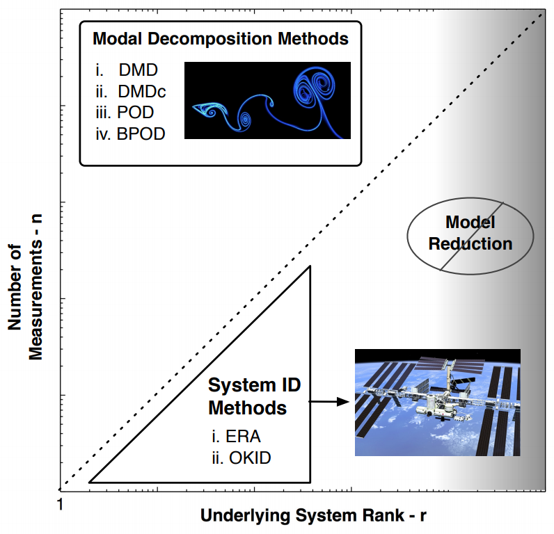
- ERA/OKID is for systems with higher dimensions than number of observables/measurements.
- DMD etc. is for systems with many observables/measurements with lower dimensional dynamics.
- ERA takes care of control input, while DMD cannot (but DMD with control, DMDc, can)
DMD v.s. EMD
Another commonly used approach is from signal processing, called Empirical Mode Decomposition (EMD), or., e.g., its more recent variant, Variational Mode Decomposition (VMD).
- Recursively decomposes a signal into different modes of unknown but separate spectral bands
- Suitable for data that is nonstationary and nonlinear.
- But mainly for 1D data (though there are multi-dimensional extensions, such as this work on unsteady aerodynamics)
Back to our example
f, ax = plt.subplots(ncols=2, figsize=(12,5))
ax[0].plot(x, dmd.modes[:,0].real, 'b-', label='DMD'); ax[0].plot(x, dmd.modes[:,1].real, 'r-')
ax[0].plot(x, -M1.real, 'k:', label='Exact'); ax[0].plot(x, M2.real, 'k:')
ax[0].legend(); ax[0].set_xlabel('x'); ax[0].set_ylabel('Mode shape'); ax[0].set_title('Modes')

ax[1].plot(t, dmd.dynamics[0].real, 'b-', label='DMD'); ax[1].plot(t, dmd.dynamics[1].real, 'r-')
ax[1].plot(t, np.real(D2), 'k:', label='Exact'); ax[1].plot(t, np.real(-D1), 'k:')
ax[1].legend(); ax[1].set_xlabel('t'); ax[1].set_ylabel('Amplitude'); _=ax[1].set_title('Dynamics')

titles = ['Mode 1', 'Mode 2', 'Reconstruction']
data = [dmd.dynamics[0].reshape(-1, 1).dot(dmd.modes[:,0].reshape(1, -1)),
        dmd.dynamics[1].reshape(-1, 1).dot(dmd.modes[:,1].reshape(1, -1)),
        dmd.reconstructed_data.T]
_=pltContours(xgrid, tgrid, data, titles)

titles = ['Residual', 'White noise', 'Uncaptured mode components']
data = [(X-dmd.reconstructed_data.T).real,
        Xn,
        (X-dmd.reconstructed_data.T-Xn).real]
_=pltContours(xgrid, tgrid, data, titles)

Pondering this example
We applied DMD to complex data, but only check the real part of reconstructed data.
- What if we directly apply DMD to the real part of the dataset?
f = plt.figure(figsize=(6,4))
plt.plot(x, dmd_real.modes[:,0], 'b--',
         label='Real only: {0:5.4f}/{1:5.4f}'.format(*_eig(dmd_real.eigs)))
plt.plot(x, dmd_real.modes[:,1], 'r--')
plt.plot(x, M1.real, 'k:',
         label='Exact: {0:5.4f}/{1:5.4f}'.format(w2, w1))
plt.plot(x, M2.real, 'k:')
plt.legend()
plt.xlabel('x')
_=plt.ylabel('Mode shape')

The real-only DMD failed like PCA, but for a different reason.
- Consider oscillation at one frequency (with or w/o damping)
- Requires a conjugate pair of two modes, i.e. modes $\boldsymbol{\phi}_{1,2}=\mathbf{u}\pm\mathbf{v}i$ with eigenvalues $\lambda_{1,2}=\zeta\pm\omega i$.
- The conjugacy can be interpreted as phase information, or "displacement v.s. velocity"
- The algorithm needs to "see" both modes in the observation - so the imag part is necessary.
- If one really wants to work with DMD within the real domain, then
- A new dataset has to be formed by stacking the real and imag parts: $\vX=[\vU^T\ \vV^T]^T$
- Number of modes requested should be doubled: One pair of (conjugate) modes correspond to one exact complex mode
- Alternatively, one could apply DMD to the real part only with a shifting, i.e., higher-order DMD
- New snapshots with $m$ shifts $\vy_k^T=[\vx_{k}^T, \vx_{k-1}^T, \cdots, \vx_{k-m}^T]$.
- There will be $(m-1)$ fewer samples.
- It essentially tries to reconstruct the missing phase/velocity data from a few snapshots within a time window.
- This technique is called Time Delayed Embedding, cf. Taken's theorem
f = plt.figure(figsize=(12,4))
plt.plot(x, _nrm(dmd.modes[:,0].real), 'b-.', label='Complex: {0:5.4f}/{1:5.4f}'.format(*_eig(dmd.eigs)))
plt.plot(x, -_nrm(dmd.modes[:,1].real), 'r-.')
plt.plot(x, -_nrm(dmd_expd.modes[:128,0]), 'b-', label='Expanded: {0:5.4f}/{2:5.4f}'.format(*_eig(dmd_expd.eigs)))
plt.plot(x, _nrm(dmd_expd.modes[:128,2]), 'r-')
plt.plot(x, -_nrm(dmd_tde.modes[:128,0]), 'b.', label='TDE: {0:5.4f}/{2:5.4f}'.format(*_eig(dmd_tde.eigs)))
plt.plot(x, -_nrm(dmd_tde.modes[:128,2]), 'r.')
plt.plot(x, dmd_real.modes[:,0], 'b--', label='Real only: {0:5.4f}/{1:5.4f}'.format(*_eig(dmd_real.eigs)))
plt.plot(x, dmd_real.modes[:,1], 'r--')
plt.plot(x, M1.real, 'k:', label='Exact: {0:5.4f}/{1:5.4f}'.format(w2, w1))
plt.plot(x, M2.real, 'k:')
plt.legend()
plt.xlabel('x')
_=plt.ylabel('Mode shape')

More discussion on DMD, and its generalization Koopman theory, in the Dynamical Systems module.
A relatively comprehensive set of DMD, from PyDMD.
