Machine Learning for Engineering

High-Dimensional System: Spatial Decomposition - Non-linear

Instructor: Daning Huang

$$ \newcommand{\norm}[1]{\left\lVert{#1}\right\rVert} \newcommand{\R}{\mathbb{R}} \newcommand{\X}{\mathcal{X}} \newcommand{\D}{\mathcal{D}} $$

TODAY: Dimension Reduction

• Autoencoder
• Variational autoencoder
• A touch on generative models

Vanilla Autoencoder

Autoencoders create general nonlinear embedding of data in a low-dimensional latent space.

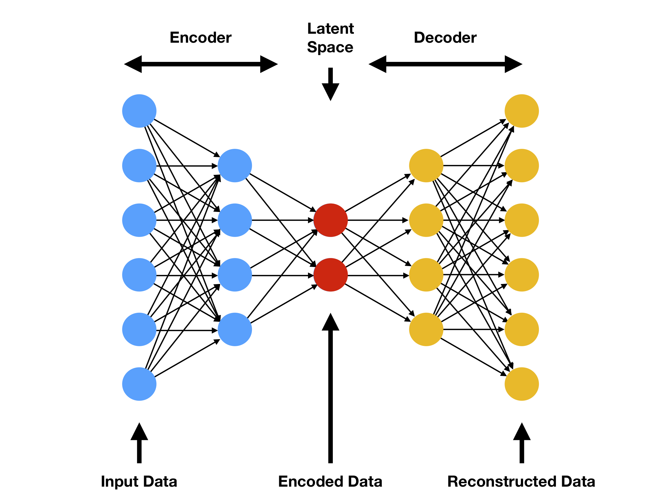
Mathematically, the model is simple

Encoder: $z=f_e(x;\theta_e)$

Decoder: $\hat{x}=f_d(z;\theta_d)$

where $\theta_e$ and $\theta_d$ are learnable parameters, and $\text{dim}(z)\ll\text{dim}(x)$.

The loss can be standard L2 norm $$ \mathcal{L}(x,\hat{x}) = \sum_{i=1}^N\norm{x_i-\hat{x}_i}^2 $$ so we minimize the error in reconstruction.

Example

We try the autoencoder on the standard MNIST dataset of hand-written digits.

plot_image(proc_image(train_loader, [0, 1, 2, 3]), sz=(12,4))

# Code inspired from https://github.com/Jackson-Kang/Pytorch-VAE-tutorial
class Encoder_AE(nn.Module):
    def __init__(self, input_dim, hidden_dim, latent_dim):
        super(Encoder_AE, self).__init__()
        self.inp1 = nn.Linear(input_dim, hidden_dim)
        self.inp2 = nn.Linear(hidden_dim, hidden_dim)
        self.ltnt = nn.Linear(hidden_dim, latent_dim)
        self.LeakyReLU = nn.LeakyReLU(0.2)

    def forward(self, x):
        _h = self.LeakyReLU(self.inp1(x))
        _h = self.LeakyReLU(self.inp2(_h))
        _h = self.ltnt(_h)
        return _h

class Decoder(nn.Module):
    def __init__(self, latent_dim, hidden_dim, output_dim):
        super(Decoder, self).__init__()
        self.hid1   = nn.Linear(latent_dim, hidden_dim)
        self.hid2   = nn.Linear(hidden_dim, hidden_dim)
        self.output = nn.Linear(hidden_dim, output_dim)
        self.LeakyReLU = nn.LeakyReLU(0.2)

    def forward(self, x):
        _h    = self.LeakyReLU(self.hid1(x))
        _h    = self.LeakyReLU(self.hid2(_h))
        x_hat = torch.sigmoid(self.output(_h))
        return x_hat

class AE(nn.Module):
    def __init__(self, Encoder, Decoder):
        super(AE, self).__init__()
        self.Encoder = Encoder
        self.Decoder = Decoder

    def forward(self, x):
        z = self.Encoder(x)
        x_hat = self.Decoder(z)
        return x_hat
    
    def predict(self, x):  # For compatibility
        return self.forward(x)

enc_ae = Encoder_AE(input_dim=x_dim, hidden_dim=hidden_dim, latent_dim=latent_dim)
dec_ae = Decoder(latent_dim=latent_dim, hidden_dim = hidden_dim, output_dim = x_dim)
mdl_ae = AE(Encoder=enc_ae, Decoder=dec_ae).to(DEVICE)

_loss = nn.MSELoss(reduction='sum')
def loss_AE(x, mdl):
    return _loss(mdl(x), x)

train_model(mdl_ae, loss_AE)

Epoch 1: 30.194967837835193
Epoch 2: 10.067500433054114
Epoch 3: 6.9388193385867725
Epoch 4: 5.7170717874313635
Epoch 5: 4.980709319202251
Epoch 6: 4.475009423257513
Epoch 7: 4.078945089859238
Epoch 8: 3.789954772337848
Epoch 9: 3.5555493169157253
Epoch 10: 3.358758305468424
Epoch 11: 3.2103049215530115
Epoch 12: 3.069630401815118
Epoch 13: 2.943403834882682
Epoch 14: 2.8330578771218633
Epoch 15: 2.74341720326317
Epoch 16: 2.6617127162825085
Epoch 17: 2.5766300531301356
Epoch 18: 2.5111068582932816
Epoch 19: 2.4387502534640255
Epoch 20: 2.385131589351393
Epoch 21: 2.3336342617028545
Epoch 22: 2.278604788804094
Epoch 23: 2.229951473739191
Epoch 24: 2.1871575828386667
Epoch 25: 2.155386094744496
Epoch 26: 2.102653617030989
Epoch 27: 2.0758359095807464
Epoch 28: 2.040510418721551
Epoch 29: 2.0098357458862917
Epoch 30: 1.9761375763499875

xtrue, xpred = eval_model(mdl_ae)    # Now we try the autoencoder on new data
idx = [0, 10, 20, 42]
plot_image(proc_image(xtrue[0], idx), sz=(8,4))
plot_image(proc_image(xpred[0], idx), sz=(8,4))

# Can we generate NEW images by interpolation in the latent space?
with torch.no_grad():
    n0, n1 = torch.randn(2, latent_dim)
    w = torch.linspace(0, 1, batch_size).reshape(-1,1)
    inp = (w*n0 + (1-w)*n1).to(DEVICE)
    generated_images = dec_ae(inp)

xs = proc_image(generated_images, [0, 19, 39, 59, 79, 99])
plot_image(xs, sz=(12,4))
# Unfortunately, no...

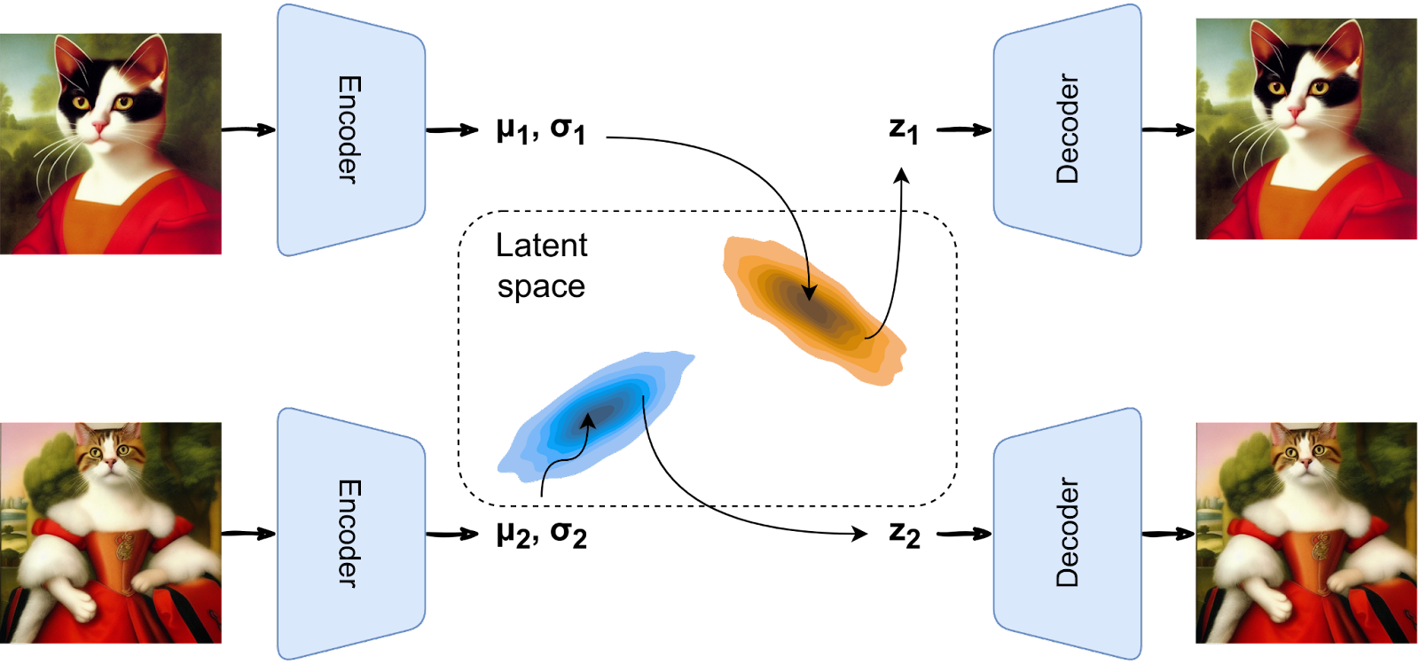
Variational AutoEncoder (VAE)

This is an initial step to the Generative Models.

Kingma et al., ArXiv 2013

Core idea: Enforce smoothness in latent space

• New encoder: $z\sim\mathcal{N}(\mu(x),\sigma^2(x))$
• Decoder remains the same: But its input $z$ is random

Figure source

Let's use probability theory to characterize the model.

Data distribution, given by dataset: $\tilde{p}(x)$

Latent distribution, assumed: $q(z)=\mathcal{N}(0,I)$

Encoder, learned: $p(z|x)=\mathcal{N}(\mu(x),\sigma^2(x))$

Decoder, learned: $q(x|z)$

• Data + Encoder give $$ p(z|x)\tilde{p}(x) = p(x,z) $$
• Latent + Decoder give $$ q(x|z)q(z) = q(x,z) $$
• The joint distribution of $x$ and $z$ should be the same $$ p(x,z) = q(x,z) $$

Use Kullback–Leibler divergence to characterize the difference. $$ KL(p||q) = \int p(x,z)\log\left(\frac{p(x,z)}{q(x,z)}\right)dxdz $$

After lengthy math $$ KL(p||q) \propto \underbrace{-\int \tilde{p}(x) \color{blue}{\log q(x|z)} dx}_{\text{Reconstruction}} + \underbrace{\int \tilde{p}(x) \color{red}{KL(p(z|x)||q(z))} dx}_{\text{Regularization}} $$

• If $q(x|z)$ is Gaussian, Reconstruction loss $\propto \norm{\hat{x}-\mu(z)}^2$; hence the name.
• Regularization enforces the encoded distribution $p(z|x)$ to be unit Gaussian.

Back to Example

class Encoder_VAE(nn.Module):
    def __init__(self, input_dim, hidden_dim, latent_dim):
        super(Encoder_VAE, self).__init__()
        self.inp1 = nn.Linear(input_dim, hidden_dim)
        self.inp2 = nn.Linear(hidden_dim, hidden_dim)
        self.mean = nn.Linear(hidden_dim, latent_dim)
        self.var  = nn.Linear(hidden_dim, latent_dim)  # New
        self.LeakyReLU = nn.LeakyReLU(0.2)

    def forward(self, x):
        h_       = self.LeakyReLU(self.inp1(x))
        h_       = self.LeakyReLU(self.inp2(h_))
        mean     = self.mean(h_)
        log_var  = self.var(h_)  # New, note that we learn log(sigma^2)
        return mean, log_var     # to ensure positivity of sigma^2
    
# class Decoder
# remains the same

class VAE(nn.Module):
    def __init__(self, Encoder, Decoder):
        super(VAE, self).__init__()
        self.Encoder = Encoder
        self.Decoder = Decoder

    def reparameterization(self, mean, var):
        # New, enables backpropagation through random samples
        epsilon = torch.randn_like(var).to(DEVICE)
        z = mean + var*epsilon
        return z

    def forward(self, x):
        mean, log_var = self.Encoder(x)
        z = self.reparameterization(mean, torch.exp(0.5 * log_var))
        x_hat = self.Decoder(z)
        return x_hat, mean, log_var        # Note the new outputs

    def predict(self, x):
        return self.forward(x)[0]

enc_va = Encoder_VAE(input_dim=x_dim, hidden_dim=hidden_dim, latent_dim=latent_dim)
dec_va = Decoder(latent_dim=latent_dim, hidden_dim = hidden_dim, output_dim = x_dim)
mdl_va = VAE(Encoder=enc_va, Decoder=dec_va).to(DEVICE)

_loss = nn.BCELoss(reduction='sum')  # Using a binary-cross-entropy loss instead
def loss_VAE(x, mdl):
    x_hat, mean, log_var = mdl(x)
    REC = _loss(x_hat, x)
    KLD = - 0.5 * torch.sum(1+ log_var - mean.pow(2) - log_var.exp())
    return REC + KLD

train_model(mdl_va, loss_VAE)

Epoch 1: 173.52214802991966
Epoch 2: 129.110544967524
Epoch 3: 116.70865482183848
Epoch 4: 112.81034709541944
Epoch 5: 110.62437705420493
Epoch 6: 108.77609867357053
Epoch 7: 107.55575478988418
Epoch 8: 106.47694948938334
Epoch 9: 105.64202525041736
Epoch 10: 105.02165815095472
Epoch 11: 104.44441283975897
Epoch 12: 103.90396427313752
Epoch 13: 103.48758464628547
Epoch 14: 103.14027183978506
Epoch 15: 102.78024919462125
Epoch 16: 102.5086123193604
Epoch 17: 102.28497179544031
Epoch 18: 102.02403370852463
Epoch 19: 101.7639648600532
Epoch 20: 101.63118320573352
Epoch 21: 101.5072508705916
Epoch 22: 101.29524319503861
Epoch 23: 101.13557287862584
Epoch 24: 101.01100639738105
Epoch 25: 100.8401448214472
Epoch 26: 100.79163619052588
Epoch 27: 100.66462023294032
Epoch 28: 100.49105137794763
Epoch 29: 100.42876656406511
Epoch 30: 100.32168006247392

xtrue, xpred = eval_model(mdl_va)    # Now we try the autoencoder on new data
idx = [0, 10, 20, 42]
plot_image(proc_image(xtrue[0], idx), sz=(8,4))
plot_image(proc_image(xpred[0], idx), sz=(8,4))

# Try to interpolate again
with torch.no_grad():
    n0, n1 = torch.randn(2, latent_dim)
    w = torch.linspace(0, 1, batch_size).reshape(-1,1)
    inp = (w*n0 + (1-w)*n1).to(DEVICE)
    generated_images = dec_va(inp)

xs = proc_image(generated_images, [0, 19, 39, 59, 79, 99])
plot_image(xs, sz=(12,4))   # We did it!

Generative Models

The decoder portion of VAE is a generative model $$ q(x|z) $$

• Randomly pick a sample from $p(z)=\mathcal{N}(0,I)$.
• Generate a new $x$ that looks like data $\tilde{p}(x)$.

There are much more architectures

• Generative Adversarial Networks (GANs)
• Autoregressive Models, e.g., PixelRNN, PixelCNN, GPT
• Normalizing Flows
• Diffusion Models
• etc.

We will cover 1-2 of these later.

One more example

"DeepSDF" model - it directly uses the latent vector to describe a 3D object.

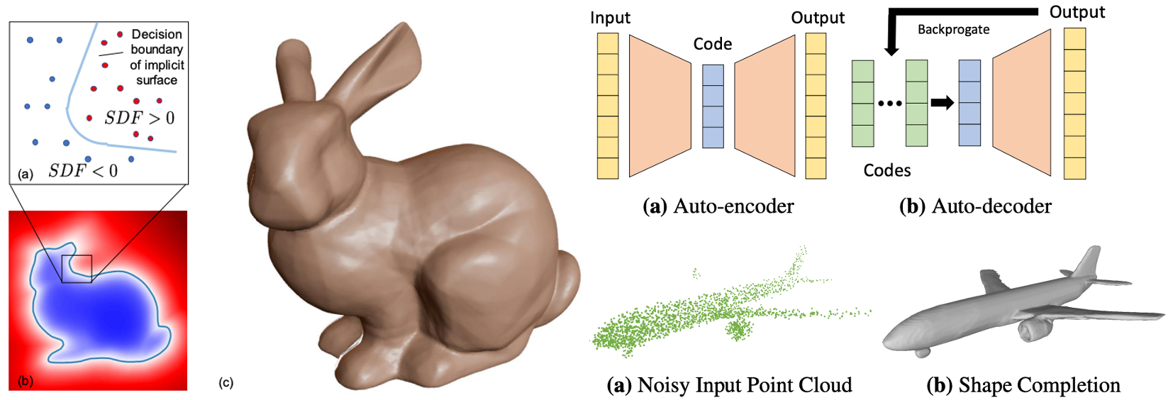
Ref: J. Park, et al., DeepSDF: Learning Continuous Signed Distance Functions for Shape Representation, 2019