Rethinking Linear Regression
Problem: Vanilla linear model $y(x) = w^T x$ can only produce straight lines/hyperplanes through the origin.
- Not very flexible / powerful
- Cannot handle nonlinearities
Solution: Regression with some features
- e.g., replace $x$ by $\phi(x) = [1, x, x^2, \cdots, x^p]^T$
- The feature mapping $\phi$ is nonlinear
- But in feature space the problem becomes linear!
Feature Mapping (or Lifting, Embedding, etc.)
Our models so far employ a nonlinear feature mapping $\phi : \mathcal{X} \mapsto \mathbb{R}^M$
- in general, features are nonlinear functions of the data
- each feature $\phi_j(x)$ extracts important properties from $x$
Ultimately, this allows us to use linear methods for nonlinear tasks.
Example
Problem: Find a linear perspective for the following scattered data.
- Left: Already linear in the current coordinates
- Right: Nonlinear - how to transform the coordinates (or, find the right features)
plot_circular_data(100)

Solution 1
Add squared-distance-to-origin $\phi(x)=(x_1^2 + x_2^2)$ as third feature.
plot_circular_3d(100)

Solution 2
Replace $(x_1, x_2)$ with $(\phi_1,\phi_2) = (x_1^2, x_2^2)$
plot_circular_squared(100)

What feature mapping does
Data has been mapped via $\phi$ to a new, higher-dimensional space
- Certain representations are better for certain problems
Alternatively, the data still lives in original space, but the definition of distance or inner product has changed.
- Certain inner products are better for certain problems
More on the second bullet soon.
Effective, but...
How do I choose a feature mapping $\phi(x)$?
- Manually? Learn features?
With $N$ examples and $M$ features,
- design matrix is $\Phi \in \mathbb{R}^{N \times M}$
- linear regression requires inverting $\Phi^T \Phi \in \mathbb{R}^{M \times M}$
- computational complexity of $O(M^3)$ - too high if too many features?
- If many features, we need many more data, so that $N\gg M$ - not always possible!
In other words, higher-dimensional features come at a price:
- We cannot manage high/infinite-dimensional $\phi(x)$.
- Computational complexity blows up.
Kernel methods to the rescue!
Kernel Functions
Many algorithms depend on the data only through pairwise inner products between data points, $$ \langle x_1, x_2 \rangle = x_2^T x_1 $$
Inner products can be replaced by Kernel Functions, capturing more general notions of similarity.
- No longer need coordinates!
Definition
A kernel function $\kappa(x,x’)$ is intended to measure the similarity between $x$ and $x’$.
So far, we have used the standard inner product in the transformed space, $$ \kappa(x, x') = \phi(x)^T \phi(x') $$
In general, $\kappa(x, x')$ is any symmetric positive-semidefinite function. This means that for every set $x_1, ..., x_n$, the matrix $[\kappa(x_i,x_j)]_{i,j\in[n]}$ is a PSD matrix.
Kernels as implicit feature map
For every valid kernel function $\kappa(x, x')$,
- there is an implicit feature mapping $\phi(x)$
- corresponding to an inner product $\phi(x)^T \phi(x')$ in some high-dimensional feature space
- And sometimes infinite dimensional!
This incredible result follows from Mercer's Theorem,
- Generalizes the fact that every positive-definite matrix corresponds to an inner product
- For more info, see Reproducing Kernel Hilbert Space (RKHS), and later in lecture.
Mapping: Equivalent to the standard inner product when either $$ \begin{gather*} \phi(x) = (x_1^2, \sqrt{2} x_1 x_2, x_2^2) \\ \phi(x) = (x_1^2, x_1 x_2, x_1 x_2, x_2^2) \end{gather*} $$
Implicit mapping is not unique, but a standard choice would be given by Mercer's theorem.
Mononomials
Kernel: Higher-order mononomial of degree $p$, $$ \kappa(x,z) = (x^T z)^p = \left( \sum_{k=1}^M x_k z_k \right)^p $$
Mapping: Implicit feature vector $\phi(x)$ contains all monomials of degree $p$
Polynomials
Kernel: Inhomogeneous polynomial up to degree $p$, for $c > 0$, $$ \kappa(x,z) = (x^T z + c)^p = \left(c + \sum_{k=1}^M x_k z_k \right)^p $$
Mapping: Implicit feature vector $\phi(x)$ contains all monomials of degree $\leq p$
Applying to CFD solutions
Take the pixel values and compute $\kappa(x,z) = (x^Tz + 1)^p $
- here, $x$ = $449 \times 129 \approx 60k$ nodes, (From NASA Langley)
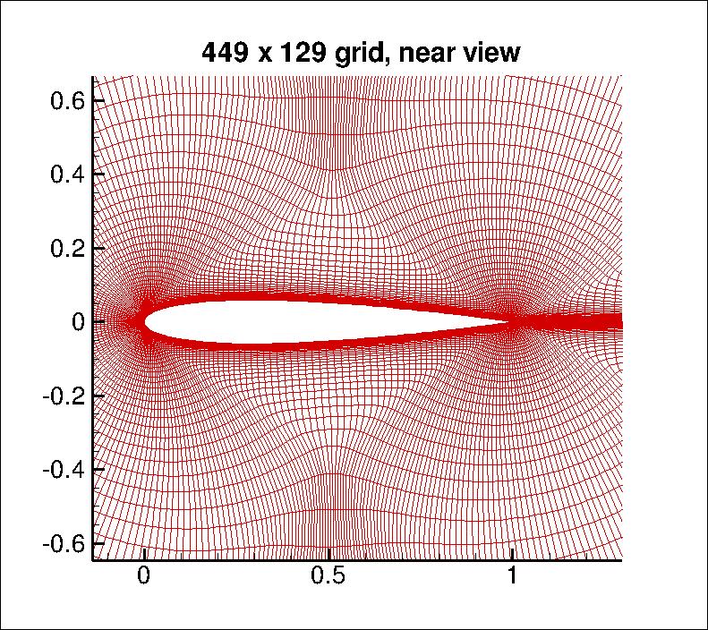
You can compute the inner product in the space of all monomials up to degree $p$
- For $dim(x)\approx 60k$ and $p=3$ a $32T$ dimensional space!
Method 2
Explicitly define a kernel $\kappa(x,x')$ and identify the implicit feature map, e.g. $$ \kappa(x,z) = (x^Tz)^2 \quad \implies \quad \phi(x) = (x_1^2, \sqrt{2} x_1 x_2, x_2^2) $$
Kernels help us avoid the complexity of explicit feature mappings.
Method 3
Define a similarity function $\kappa(x, x')$ and use Mercer's Condition to verify that an implicit feature map exists without finding it.
- Define the Gram matrix $K$ to have elements $K_{nm} = \kappa(x_n,x_m)$
- $K$ must positive semidefinite for all possible choices of the data set {$x_n$} $$ a^TKa \equiv \sum_{i}\sum_{j} a_i K_{ij} a_j \geq 0 \quad \forall\, a \in \mathbb{R}^n $$
Building Blocks
There are a number of axioms that help us construct new, more complex kernels, from simpler known kernels.
- For kernels $\kappa_1$ and $\kappa_2$, and a positive scalar $s$, then the following are kernels too:
$$ \kappa_1+\kappa_2,\quad s\kappa_1,\quad \kappa_1\kappa_2 $$
You will prove some specific cases in homework
- For example, the following are kernels: $$ \begin{align*} \kappa(x, x') &= f(x) \kappa_1(x,x') f(x') \\ \kappa(x, x') &= \exp( \kappa_1(x, x') ) \end{align*} $$
Popular Kernel Functions
Simple Polynomial Kernel (terms of degree $2$) $$\kappa(x,z) = (x^Tz)^2 $$
Generalized Polynomial Kernel (degree $M$) $$\kappa(x,z) = (x^Tz + c)^M, c > 0 $$
Gaussian Kernels $$ \kappa(x,z) = \exp \left\{-\frac{\|x-z\|^2}{2\sigma^2} \right\} $$
Particularly for Gaussian Kernel
Not related to Gaussian PDF!
Translation invariant (depends only on distance between points)
Corresponds to an infinitely dimensional space!
The Kernel Trick
What kernels essentially do
- Compute inner products in a high dimensional space (i.e., $\phi$).
- But with only the computational cost of a low dimensional space (i.e., $x$).
What kernel trick does
- Many algorithms can be expressed completely in kernels/inner products $\kappa(x,x’)$, rather than other operations on $x$, e.g., $\phi(x)$.
- Huge reduction in cost ($x$ instead of $\phi$), but still with high expressibility ($\phi$).
Example: Similarity
Conventionally the similarity between two points $x$ and $z$ can be quantified as the "angle" between vectors $$ s(x,z) = \frac{x^T z}{\|x\|\|z\|} $$
In feature space, we can generalize as $$ s(x,z) = \frac{\phi(x)^T \phi(z)}{\|\phi(x)\|\|\phi(z)\|} $$
But this is simply $$ s(x,z) = \frac{k(x,z)}{\sqrt{k(x,x)k(z,z)}} $$
Example: Distance
Distance between samples can be expressed in inner products: $$ \begin{align*} \|\phi(x) - \phi(z) \|^2 &= \langle\phi(x)- \phi(z), \phi(x)- \phi(z) \rangle\\ &= \langle \phi(x), \phi(x)\rangle - 2\langle\phi(x), \phi(z)\rangle + \langle\phi(z), \phi(z) \rangle \\ &= \kappa(x,x) - 2\kappa(x,z) + \kappa(z,z) \end{align*} $$
Example: Distance to the Mean
Mean of data points given by: $\phi(s) = \frac{1}{N}\sum_{i=1}^{N}\phi(x_i)$
Distance to the mean: $$ \begin{align*} \|\phi(x) - \phi_s \|^2 &= \langle\phi(x)- \phi_s, \phi(x)- \phi_s \rangle\\ &= \langle \phi(x), \phi(x)\rangle - 2\langle\phi(x), \phi_s\rangle + \langle\phi_s, \phi_s \rangle \\ &= \kappa(x,x) - \frac{2}{N}\sum_{i=1}^{N}\kappa(x,x_i) + \frac{1}{N^2}\sum_{j=1}^{N}\sum_{i=1}^{N}\kappa(x_i,x_j) \end{align*} $$
Example: Ridge Regression
This is the main goal for this lecture, see next ...
Kernelizing the Ridge Regression
Recall ...
Linear Regression Model $$ y(x,w) = w^T \phi (x) = \sum_{j=0}^{M} w_j \phi_j(x) $$
Ridge Regression $$ J(w) = \frac{1}{2} \sum_{n=1}^{N}(w^T \phi (x_n) - t_n)^2 + \frac{\lambda}{2}w^Tw $$
Closed-form Solution $$ w = (\Phi^T \Phi + \lambda I)^{-1}\Phi^T t $$
Dualization
We want to minimize: $J(w) = \frac{1}{2} \sum_{n=1}^{N}(w^T \phi (x_n) - t_n)^2 + \frac{\lambda}{2}w^Tw$
Taking $\nabla J(w) = 0$, we obtain: $$ \begin{align*} w &= -\frac{1}{\lambda}\sum_{n=1}^{N}(w^T\phi(x_n) - t_n) \phi(x_n) \\ &\equiv \sum_{n=1}^{N}a_n\phi(x_n) = \Phi^Ta \end{align*} $$ Notice: $w$ can be written as a linear combination of $\phi(x_n)$!
Transform $J(w)$ to $J(a)$ by substituting $ w = \Phi^T a$
- Where $a_n = -\frac{1}{\lambda}\left(w^T\phi(x_n) - t_n\right)$
- Let $a = (a_1, \dots, a_N)^T$ be the parameter, instead of $w$.
Dual Representation
Substituting $w = \Phi^Ta$, $$ \begin{align*} J(a) &= \frac12 w^T \Phi^T \Phi w - w^T \Phi^T t + \frac12 t^T t + \frac{\lambda}{2} w^T w \\ &= \frac{1}{2} (a^T\Phi) \Phi^T \Phi (\Phi^Ta) - (a^T\Phi) \Phi^Tt + \frac{1}{2}t^Tt + \frac{\lambda}{2}(a^T\Phi)(\Phi^Ta) \\ &= \frac{1}{2} a^T {\color{red}{(\Phi \Phi^T) (\Phi \Phi^T)}} a - a^T {\color{red}{(\Phi\Phi^T)}} t + \frac{1}{2}t^Tt + \frac{\lambda}{2}a^T {\color{red}{(\Phi\Phi^T)}} a \\ &= \frac{1}{2}a^TKKa - a^T Kt + \frac{1}{2}t^Tt + \frac{\lambda}{2}a^TKa \end{align*} $$
More concisely, $$ J(a) = \|Ka-t\|_2^2 + \lambda \|a\|_K^2 $$
- The first term is the usual prediction error
- The second term is a "K-norm", which is technically the RKHS norm - it controls smoothness.
- The solution is
$$ {a = (K+\lambda I_N)^{-1}t} $$
The predictive model becomes $$ y(x) = w^T\phi(x) = a^T \Phi\phi(x) = a^T k(x) $$ where $$ k(x) = \Phi \phi(x) = [\kappa(x_1,x), \kappa(x_2,x), \ldots, \kappa(x_N,x)]^T $$
- We have gotten rid of all $\phi$!
Comparison
Primal - Ridge Regression: $w = (\Phi^T\Phi + \lambda I_M)^{-1} \Phi^Tt $
- invert $\Phi^T \Phi \in \mathbb{R}^{M \times M}$
- cheaper since usually $N \gg M$
- must explicitly construct features
Dual - Kernel Ridge Regression: $ a = (K + \lambda I_N)^{-1}t $
- invert Gram matrix $K \in \mathbb{R}^{N \times N}$
- use kernel trick to avoid feature construction
- use kernels $\kappa(x, x')$ to represent similarity over vectors, images, sequences, graphs, text, etc..
Kernel Ridge Regression: Example
# Tries to match everything, but no severe overfitting
plot_kernel_ridge(X, y, gamma=4, lmbd=0.01, ker='rbf')

Larger penalty
# Smoother and less variation
plot_kernel_ridge(X, y, gamma=4, lmbd=0.5, ker='rbf')

Smaller bandwidth
$\kappa(x,y)=\exp(-\gamma\|x-y\|^2)$
# More localized
plot_kernel_ridge(X, y, gamma=10, lmbd=0.01)

Changing kernel
"linear": $\kappa(x,y)=x^Ty$
# Effectively a regularized linear fit
plot_kernel_ridge(X, y, gamma=4, lmbd=0.5, ker='linear')

Two More Perspectives
Kernel itself as features
For a dataset $\{x_i\}_{i=1}^N$, pick a kernel $\kappa$ and define features as $$ \tilde{\phi}_i(x) = \kappa(x,x_i) $$ i.e., each sample corresponds to one feature.
The KRR model is $$ y(x) = \sum_{i=1}^N a_i\kappa(x,x_i) \equiv \tilde{\phi}(x)^T a $$
So we could have treated KRR as a regular ridge regression.
- In fitting, $\tilde{\phi}_i$ forms a $\Phi$ that is exactly $K$.
- The difference: the regularization in KRR $\|a\|_K^2$ but RR would use $\|a\|_2^2$.
This view has a deep connection to the Reproducing Kernel Hilbert Space (RKHS).
- The collection $\{f(x) \mid f(x)=\sum_{i=1}^N a_i\kappa(x,x_i),\, a_i\in\mathbb{R}\}$ is a function space
- Upon "completion", the space becomes RKHS
- The many nice properties of RKHS guarantee the nice properties of KRR
See the theoretical slides for more details.
Bias-variance trade-off
Recall from Ridge Regression with $m$ features and $n$ data points, we had $$ \mathbb{E}[(y - \hat{f})^2] = \underbrace{O({\sigma^2})}_\text{irreducible error} + \underbrace{O(\sigma^2\frac{{\tilde{m}}}{n})}_\text{Variance} + \underbrace{O({\tilde{m}}^{-p})}_{\text{Bias}^2} $$ where the effective number of features were introduced $$ {\tilde{m}} = \sum_{j=1}^m \frac{\nu_i}{\nu_i+\lambda} $$ and $\nu_i$'s are the eigenvalues of $\Phi^\top\Phi$.
- For $d$-dimensional input $x$ and $p$th-order polynomial features: $m\sim d^p$
- $m$ explodes for even moderate $d$ and $p$.
- Huge variance would be introduced.
Now in Kernel version, we effectively have $m=n$ features instead
- so $\nu_i$'s are the eigenvalues of $K$.
- and $$ \text{Variance}\sim \frac{\tilde{m}}{n} < 1\quad\rightarrow\text{Under control!} $$
Side Note: Locally-Weighted Linear Regression
LWLR is also frequently used. It "looks like" but is not KRR.
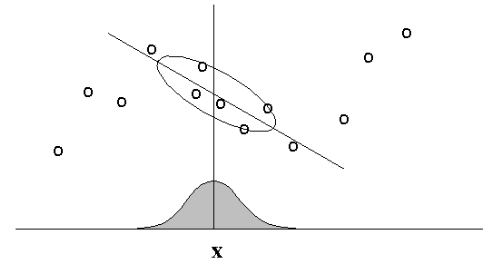
Main Idea: When predicting $f(x)$, give high weights for neighbors of $x$.
Regular vs. Locally-Weighted Linear Regression
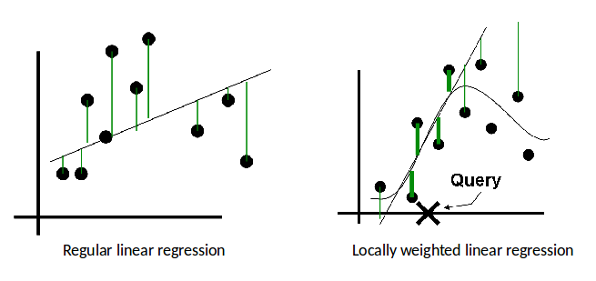
Linear Regression
2. Output $w^T \phi(x_k)$
Locally-weighted Linear Regression
2. Output $w^T \phi(x_k)$
- The standard choice for weights $r$ uses the Gaussian Kernel, with kernel width $\tau$ $$ r_k = \exp\left( -\frac{|| x_k - x ||^2}{2\tau^2} \right) $$
- Note $r_k$ depends on both $x$ (query point); must solve linear regression for each query point $x$.
- Can be reformulated as a modified version of least squares problem.
- Choice of kernel width matters.
- (requires hyperparameter tuning!)
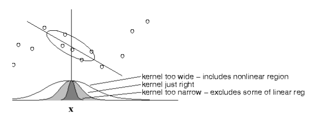
The estimator is minimized when kernel includes as many training points as can be accomodated by the model. Too large a kernel includes points that degrade the fit; too small a kernel neglects points that increase confidence in the fit.
KRR v.s. LWLR: Similarities
Both methods are “instance-based learning”, i.e., non-parametric method
- Only observations (training set) close to the query point are considered (highly weighted) for regression computation.
- Kernel determines how to assign weights to training examples (similarity to the query point x)
- Free to choose types of kernels
- Both can suffer when the dataset size is large.
KRR v.s. LWLR: Differences
- LWLR: Weighted regression; slow, but more accurate
- KRR: Weighted mean; faster, but less accurate