Machine Learning for Engineering

Kernels and Gaussian Processes: Probabilitic Formulation

Instructor: Daning Huang

$$ \newcommand{\GP}{\mathcal{GP}} \newcommand{\cD}{\mathcal{D}} \newcommand{\cF}{\mathcal{F}} \newcommand{\cL}{\mathcal{L}} \newcommand{\cN}{\mathcal{N}} \newcommand{\cb}{\mathcal{b}} \newcommand{\tcL}{\tilde{\mathcal{L}}} \newcommand{\vA}{\mathbf{A}} \newcommand{\vB}{\mathbf{B}} \newcommand{\vC}{\mathbf{C}} \newcommand{\vD}{\mathbf{D}} \newcommand{\vF}{\mathbf{F}} \newcommand{\vH}{\mathbf{H}} \newcommand{\vI}{\mathbf{I}} \newcommand{\vK}{\mathbf{K}} \newcommand{\vL}{\mathbf{L}} \newcommand{\vM}{\mathbf{M}} \newcommand{\vO}{\mathbf{O}} \newcommand{\vQ}{\mathbf{Q}} \newcommand{\vR}{\mathbf{R}} \newcommand{\vU}{\mathbf{U}} \newcommand{\vV}{\mathbf{V}} \newcommand{\vX}{\mathbf{X}} \newcommand{\vb}{\mathbf{b}} \newcommand{\vg}{\mathbf{g}} \newcommand{\vh}{\mathbf{h}} \newcommand{\vg}{\mathbf{g}} \newcommand{\vl}{\mathbf{l}} \newcommand{\vm}{\mathbf{m}} \newcommand{\vx}{\mathbf{x}} \newcommand{\vy}{\mathbf{y}} \newcommand{\tvD}{\tilde{\mathbf{D}}} \newcommand{\tvK}{\tilde{\mathbf{K}}} \newcommand{\tvb}{\tilde{\mathbf{b}}} \newcommand{\tvg}{\tilde{\mathbf{g}}} \newcommand{\vKyi}{\mathbf{K}_y^{-1}} \newcommand{\tKyi}{\tilde{\mathbf{K}}_y^{-1}} \newcommand{\sfs}{\sigma_f^2} \newcommand{\sns}{\sigma_n^2} \newcommand{\tsn}{\tilde{\sigma}_n^2} \newcommand{\half}{\frac{1}{2}} $$

TODAY: Kernels and GP - II

• Historical background: kriging
• Multivariate correlation
• Gaussian process
• Probabilistic formulation
• Determination of hyperparameters

References

• GPML Chps. 1, 2, 4, 5
• DACE Toolbox Manual

"Kriging" model by Danie G. Krige

Danie Gerhardus Krige (26 August 1919 – 3 March 2013), South African statistician and mining engineer who pioneered the field of geostatistics. Inventor of kriging.

$$ y=\underbrace{f(x)}_{Trend}+\underbrace{e(x)}_{Noise} $$

• Capture the global trend of a dataset, such that the error behaves like white noise.
• But now the noise is location-depedent.

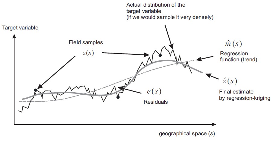
Now kriging is more or less the same as "Gaussian process regression" (GPR)

• GPR can be viewed as the probabilistic version of KRR
• GPR is our focus in this lecture

Correlation and Covariance

Covariance function

# Spatial correlation between Gaussian samples at different locations
a = [0.0, 0.0]
x, RV, KS = genGPsmp(5,     # Number of sampling points
                     0.05,  # Length scale in a SE correlation term
                     a,     # Coefficients of second-order polynomial
                     1000)  # Number of GP realizations
plt.figure()
plt.imshow(KS)
plt.colorbar()
_=pltCorr(x, RV)
_=pltGPsmp(x, RV, a,
           bnd=True,        # Plot error bounds
           smp=True)

# Realizations over a set of sampling points
a = [10.0, 0.0]
x, RV, _ = genGPsmp(200,           # Number of sampling points
                    0.0025,        # Length scale in a SE correlation term
                    a,             # Coefficients of second-order polynomial
                    1000)          # Number of GP realizations
_=pltGPsmp(x, RV, a,
           bnd=True,               # Plot error bounds
           smp=True)               # Highlight three samples and plot the mean

Gaussian Process

From wikipedia:

• A stochastic process is a collection of random variables indexed by time or space
• A Gaussian process (GP) is a stochastic process, such that every finite collection of those random variables has a multivariate Gaussian distribution

We say a function subjects to a GP, $$ f(\vx) \sim \GP(m(\vx),k(\vx,\vx')) $$ where $m(\vx)$ is the mean function and $k(\vx,\vx')$ is the covariance function, when $$ \begin{aligned} m(\vx) &= \mathrm{E}[f(\vx)] \\ k(\vx,\vx') &= \mathrm{E}[(f(\vx)-m(\vx))(f(\vx')-m(\vx'))] \end{aligned} $$ The probabilistic distribution of a set of points $\cD=\{ \vX,\vy\}$ sampled from GP is Gaussian, $$ \vy\sim\cN(\vm,\vK) $$ where $[\vm]_i=m(\vX_i)$ and $[\vK]_{ij}=k(\vX_i,\vX_j)$.

Covariance function

A covariance function of a Gaussian process is defined as, $$ k(\vx_i,\vx_j) = \sfs R(\vx_i,\vx_j) $$ where

• $\sfs$ is the process variance
• $R$ is typically stationary, i.e. $R(\vx,\vx')=R(\vx-\vx')$, and monotonically decreasing.
• Also assuming $R(0)=1$, meaning that a point correlates with itself the most.

When the observation is noisy, the covariance function is modified as, $$ k(\vx_i,\vx_j) = \sfs R(\vx_i,\vx_j) + \sns \delta_{ij} \equiv \sfs [R(\vx_i,\vx_j) + \tsn \delta_{ij}] $$

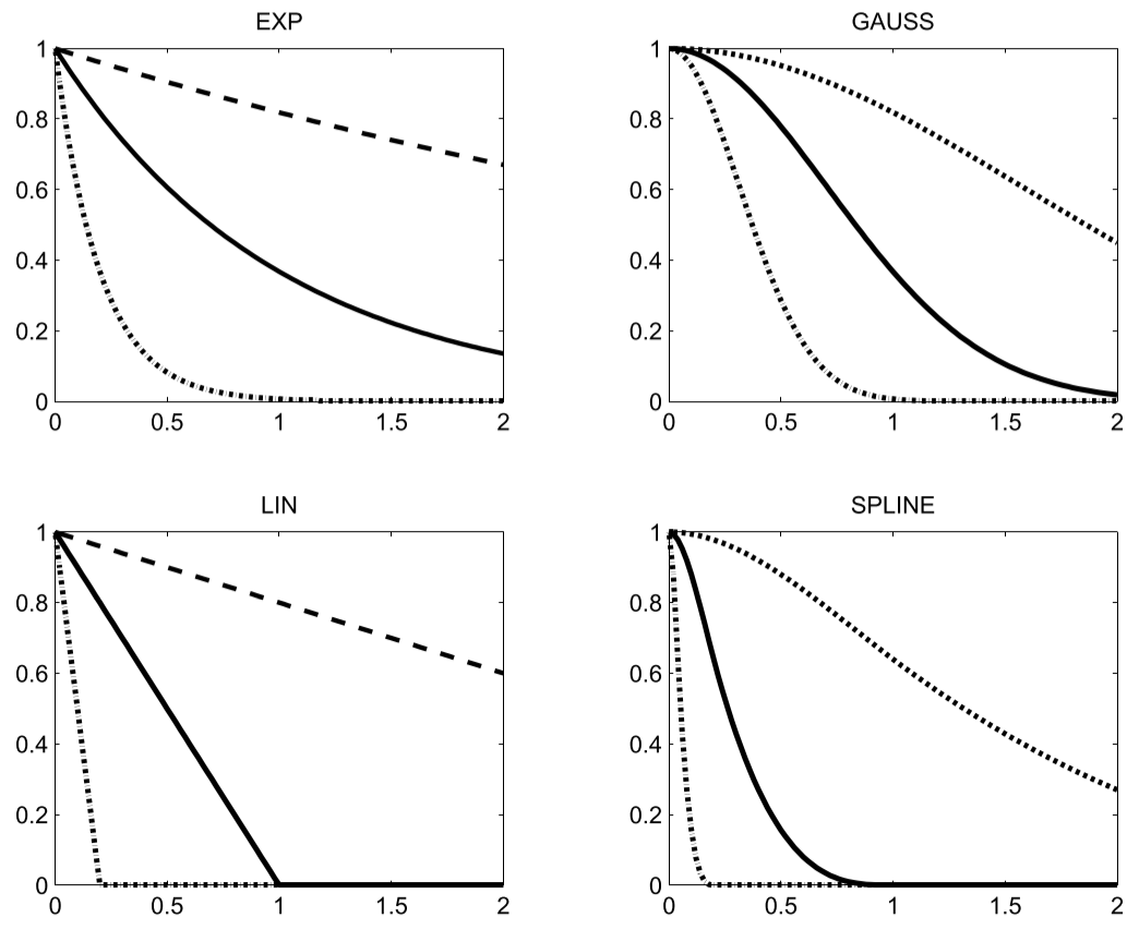
Some possible covariance functions ($r=||\vx-\vx'||$)

• Squared exponential (More discussion later) $$ k(r) = \exp\left(-\frac{r^2}{l^2}\right) $$
• Matérn class: $$ k(r) = \frac{2^{1-\nu}}{\Gamma(\nu)} \left(\frac{\sqrt{2\nu}r}{l}\right)^\nu K_\nu \left(\frac{\sqrt{2\nu}r}{l}\right) $$
• Piecewise polynomial, e.g. $$ k(r) = (1-r)_+^j[(j+1)r+1] $$ where $j$ depends on dimension, and it has a "compact support", i.e. non-zero within limited range.
• Periodic kernels, e.g. $$ k(r) = \cos\left(\frac{r}{l}\right) $$

# Example covariance functions
N = 1001
r = 0.1
X = np.linspace(0,1,N)
figure = plt.figure(figsize=(6,4))
plt.plot(X, SEKernel(X,r), 'b-', label='Squared Exponential')
plt.plot(X, M3Kernel(X,r), 'r-', label='Matern 3/2')
plt.plot(X, PPKernel(X,r), 'k-', label='Piecewise Polynomial')
plt.plot(X, CosKernel(X,r), 'm--', label='Cos')
plt.xlabel('r')
plt.ylabel("Cov")
_=plt.legend(loc=0)

# Example realizations of GPs with different covariance functions
figure = plt.figure(figsize=(6,4))
plt.plot(X, S_SE, 'b-', label='Squared Exponential')
plt.plot(X, S_MT, 'r-', label='Matern 3/2')
plt.plot(X, S_PP, 'k-', label='Piecewise Polynomial')
plt.plot(X, S_CS, 'm--', label='Cosine')
plt.xlabel("X")
plt.ylabel("SAMPLE")
_=plt.legend(loc=0)

A typical choice of $R$ is the squared exponential function, $$ R(\vx_i,\vx_j) = \exp[-(\vx_i-\vx_j)^T\vM(\vx_i-\vx_j)] $$ where in the isotropic case, $\vM=\frac{1}{2l^2}\vI$ meaning that the length scales in all dimensions are the same; while in the anisotropic case, $\vM=\half diag(\vl)^{-2}$ is a diagonal matrix with positive diagonal entries, representing the length scales in different dimensions.

Hyperparameters so far:

• Length scales $\vl$ - to be found by automatic relevance determination (ARD)
• Variances $\sfs$ and $\sns$

The basic form

Return to the dataset $\cD=\{ \vX,\vy\}$ sampled from GP: $$ \vy\sim\cN(\vm,\vK) $$ where $[\vm]_i=m(\vX_i)$ and $[\vK]_{ij}=k(\vX_i,\vX_j)$. Note that scalar output is assumed.

Now split the points into two sets: the training set $\vX_s$ with known output $\vy_s$, and the target set $\vX_u$ with unknown output $\vy_s$. The joint distribution is still Gaussian, with the following mean, $$ \vm^T = [\vm(\vX_s)^T, \vm(\vX_u)^T] \equiv [\vm_s^T, \vm_u^T] $$ and the block covariance matrix, $$ \vK = \begin{bmatrix} \vK_{ss} & \vK_{su} \\ \vK_{us} & \vK_{uu} \end{bmatrix} $$ where the $i,j$th element of $\vK$ is associated with the $i$th and $j$th rows of $\vX$, $$ [\vK_{ab}]_{ij} = k([\vX_a]_i, [\vX_b]_j) $$

When $\vy_s$ is noisy, a white noise term with variance $\sigma_n^2$ is added to the Gaussian distribution, adding a diagonal matrix to $\vK_{ss}$ $$ \vK_y = \vK_{ss} + \sigma_n^2 \vI_{ss} $$

Prediction and error estimate

The distribution of $\vy_u$ given $\vy_s$ is found by conditional probability, $$ \vy_u|\vy_s \sim \cN(\vm_p, \vK_p) $$ where the predictive mean is, $$ \vm_p = \vm_u + \vK_{us}\vK_y^{-1}(\vy_s-\vm_s) $$ and the (predictive) covariance is, $$ \vK_p = \vK_{uu} - \vK_{us}\vK_y^{-1}\vK_{su} $$

What are the differences between the predictive mean and the kernel ridge formulation?

• If the mean function is zero, $\vm_p$ is exactly the KRR, and $\sigma_n^2$ is the penalty term! $$ \vm_p = \vK_{us}(\vK_{ss} + \sigma_n^2 \vI_{ss})^{-1}\vy_s $$
• In this case, the covariance provides the uncertainty bound.

Same idea as linear regression v.s. its probablistic version - but more flexible variance distribution

# Posterior GP's
data = np.array([
    [0.2, 0.4, 0.8],   # Input
    [0.8,-0.2, 0.2]    # Output
])
mp, std, fp = genGP(X, data, SEKernel, r, nsmp=5)
plotGP(X, data, mp, std, fp)

Using basis functions for the mean function

The form of mean function is usually unknown beforehand, so it is more common to use a set of basis functions, $$ m(\vx) = \vh(\vx)^T\cb $$ The coefficients $\cb$ have to be fitted from the sample data. Under a Bayesian framework, $\cb$ is assumed to subject to, $$ \cb \sim \cN(\vb, \vB) $$ Taking $\cb$ into account, the GP is modified as, $$ f(\vx) \sim \GP(\vh(\vx)^T\vb,k(\vx,\vx')+\vh(\vx)^T\vB\vh(\vx)) $$ Extra terms due to the basis functions shall be added to the covariance matrix, $$ \vK_{ab} = \vK(\vX_a, \vX_b) + \vH_a \vB \vH_b^T,\quad [\vH_*]_i=\vh([\vX_*]_i)^T $$

With that, we arrive at the commonly used form of GPR, $$ \begin{aligned} \vm_p^* &= \vK_{us}\vKyi\vy_s + \vD^T (\vH^T\vKyi\vH)^{-1} \vH\vKyi\vy_s \\ &= \vK_{us}\bar\vg + \vH_u\bar\vb \\ \vK_p^* &= \vK_p + \vD^T (\vH^T\vKyi\vH)^{-1} \vD \end{aligned} $$ where $\bar\vb=(\vH^T\vKyi\vH)^{-1}\vH^T\vKyi\vy_s$ and $\bar\vg=\vKyi(\vy_s-\vH\bar\vb)$. The term $\bar\vb$ is essentially the coefficients of the mean function fitted from the sample data. Also, note that some people argue that the last term in $\vK_p^*$ can neglected for simplicity [Sasena2002].

Details of derivation: Skip in class -->

Simplification

The extra terms make the predictive mean and covariance from the previous section extremely cumbersome to compute. Simplifications are needed and enabled by invoking the matrix inversion lemma, $$ (\vA+\vU\vC\vV^T)^{-1} = \vA^{-1} - \vA^{-1}\vU (\vC^{-1}+\vV^T\vA^{-1}\vU)^{-1} \vV^T\vA^{-1} $$

In current case, the lemma is applied as follows, $$ (\vK_y + \vH \vB \vH^T)^{-1} = \vKyi-\vKyi\vH \vC^{-1} \vH^T \vKyi \equiv \vKyi-\vA $$

where $\vC=\vB^{-1} + \vH^T \vKyi \vH$ and the subscript $s$ is dropped in $\vH_s$. Furthermore, the following identities can be derived, $$ \begin{aligned} \vB\vH^T(\vKyi-\vA) &= \vC^{-1}\vH^T\vKyi \\ (\vKyi-\vA)\vH\vB &= \vKyi\vH\vC^{-1} \end{aligned} $$ The simplification procedure is bascally to cancel out matrices by combining the $\vH$ and $(\vKyi-\vA)$ terms.

The predictive mean is simplified to, $$ \begin{aligned} \vm_p^* &= \vH_u\vb + (\vK_{us} + \vH_u\vB\vH^T)(\vK_y + \vH\vB\vH^T)^{-1}(\vy_s-\vH\vb) \\ &= \vK_{us}\vKyi\vy_s + \vD^T \vC^{-1} (\vH^T \vKyi \vy_s + \vB^{-1}\vb) \end{aligned} $$ where $\vD=\vH_u^T-\vH^T \vKyi \vK_{su}$. The covariance matrix is simplied to, $$ \begin{aligned} \vK_p^* &= \vK_{uu} + \vH_u\vB\vH_u^T - (\vK_{us}+\vH_u\vB\vH^T) (\vK_y + \vH\vB\vH^T)^{-1} (\vK_{su}+\vH\vB\vH_u^T) \\ &= \vK_p + \vD^T \vC^{-1} \vD \end{aligned} $$

Finally, consider the case that the coefficients are distributed uniformly, instead of Gaussian. That means $\vb\rightarrow\mathrm{0}$ and $\vB^{-1}\rightarrow \vO$. Then we arrive at the common form of GP shown earlier.

<-- Skip in class

Details of derivation: Skip in class -->

Computational aspects

The computation of $\vm_p^*$ and $\vK_p^*$ can be tricky due to the ill-conditioned matrix inversion. The strategy is to combine cholesky decomposition and QR decomposition to stabilize the inversions, i.e. $\vK_y^{-1}$ and $(\vH^T\vKyi\vH)^{-1}$.

For inversion of $\vK_y$, $$ \vKyi\vx = (\vL\vL^T)^{-1}\vx = \vL^{-T} (\vL^{-1}\vx) $$ where $\vL$ is a lower triangular matrix, and the matrix inversion is converted to two consecutive triangular solves.

To inverse $\vH^T\vKyi\vH$, $$ \vH^T\vKyi\vH = (\vL^{-1}\vH)^T (\vL^{-1}\vH) \equiv \vF^T\vF = \vR^T\vR $$ where QR decomposition is used $\vQ\vR=\vF$, $\vQ$ is an orthogonal matrix, and $\vR$ is an upper triangular matrix. $\vQ$ is tall and slim, because the number of rows equals to the number of samples, while the number of columns equals to the number of basis functions.

After the stabilization, the quantities $\bar\vb$ and $\bar\vg$ in $\vm_p^*$ are computed as follows, $$ \begin{aligned} \bar\vb &= (\vH^T\vKyi\vH)^{-1}\vH^T\vKyi\vy_s = \vR^{-1} [\vQ^T(\vL^{-1}\vy_s)] \\ \bar\vg &= \vKyi(\vy_s-\vH\bar\vb) = \vL^{-T} [\vL^{-1} (\vy_s-\vH\bar\vb)] \end{aligned} $$

The covariance matrix is computed as follows, $$ \vK_p^* = \vK_{uu} - (\vL^{-1}\vK_{su})^2 + (\vR^{-T} [\vH_u^T - \vF^T(\vL^{-1}\vK_{su})])^2 $$ where $(\Box)^2=\Box^T\Box$.

<-- Skip in class

Are we done yet?

Yes...?

No, how about hyperparameters?

• Length scales $\vl$ in the covariance functions
• Process variance $\sfs$
• Process noise $\sns$
  • Determined by measurement
  • Zero if using computer simulations, but typical people use a small value for numerical stability

Preprocessing - Non-dimensionalization

For easier treatment, we non-dimensionalize some quantities in the GPR model.

The covariance matrices $\vK_y$ and $\vK_{su}$ can be "non-dimensionalized" by $\sfs$, $$ \begin{aligned} \vK_y &\equiv \sfs \tvK_y \equiv \sfs (\tvK_{ss} + \tsn\vI) \\ \vK_{su} &\equiv \sfs \tvK_{su} \end{aligned} $$

Subsequently, for the predictive mean, $$ \vm_p^* = \vK_{su}^T\bar\vg + \vH_u^T\bar\vb = \tvK_{su}^T\tvg + \vH_u^T\tvb $$

Details of derivation: Skip in class -->

where, $$ \begin{aligned} \bar\vb &= (\vH^T\vKyi\vH)^{-1}\vH^T\vKyi\vy_s = (\vH^T\tKyi\vH)^{-1}\vH^T\tKyi\vy_s \equiv \tvb\\ \bar\vg &= \vKyi(\vy_s-\vH\bar\vb) = \sigma_f^{-2} \tKyi(\vy_s-\vH\tvb) \equiv \sigma_f^{-2} \tvg \end{aligned} $$ And the covariance, $$ \begin{aligned} \vK_p^* &= \vK_{uu} - \vK_{us}\vK_y^{-1}\vK_{su} + \vD^T (\vH^T\vKyi\vH)^{-1} \vD \\ &= \sfs [\tvK_{uu} - \tvK_{us}\tKyi\tvK_{su} + \tvD^T (\vH^T\tKyi\vH)^{-1} \tvD] \end{aligned} $$ where, $$ \vD = \vH_u^T-\vH^T \vKyi \vK_{su} = \vH_u^T-\vH^T \tKyi \tvK_{su} \equiv \tvD $$ In sum, $\sfs$ has no direct effect on the mean, but the covariance is proportional to $\sfs$, once the length scales are given.

<-- Skip in class

Learning the hyperparameters

Log-likelihood

The hyperparameters are determined using the maximum likelihood estimation (MLE). With the joint Gaussian distribution, the log marginal likelihood of the training data is, $$ \begin{aligned} \cL &= \log p(\vy_s|\vX_s,\vb,\vB) \\ &= - \half(\vy_s-\vH\vb)^T (\vK_y+\vH^T\vB\vH)^{-1} (\vy_s-\vH\vb) \\ &- \half \log |\vK_y+\vH^T\vB\vH| - \frac{n}{2}\log 2\pi \end{aligned} $$ where $n$ is number of training data points.

Factor $\cL$ with $\sfs$, $$ -2\tcL_1 = \sigma_f^{-2} (\vy_s - \vH\tvb)^T \tKyi (\vy_s - \vH\tvb) + \log|\tvK_y| + \log|\vH^T\tKyi\vH| + (n-m)\log\sfs $$ where the constant term is neglected.

If the prior on the coefficients of the basis functions is ignored, the log-likelihood simplifies to, $$ -2\tcL_2 = \sigma_f^{-2} (\vy_s - \vH\tvb)^T \tKyi (\vy_s - \vH\tvb) + \log|\tvK_y| + n\log\sfs $$

Details of derivation: Skip in class -->

Utilizing the determinant counterpart of matrix inversion lemma, $$ |\vA+\vU\vC\vV^T| = |\vA| |\vC| |\vC^{-1} + \vV^T\vA^{-1}\vU| $$ and let $\vb=0$ and $\vB^{-1}\rightarrow\vO$ as was done last time, $$ -2\cL = \vy_s^T [\vKyi - \vKyi\vH (\vH^T\vKyi\vH)^{-1} \vH^T \vKyi] \vy_s + \log|\vK_y| + \log|\vH^T\vKyi\vH| + (n-m)\log 2\pi $$ where $m$ is number of basis functions, and was introduced due to the singularity caused by $|\vB|$.

An interesting simplification can be done to the first term in the above expression, $$ \begin{aligned} I_1 &= \vy_s^T [\vKyi - \vKyi\vH (\vH^T\vKyi\vH)^{-1} \vH^T \vKyi] \vy_s \\ &= \vy_s^T \vKyi (\vy_s - \vH\bar\vb) \equiv I_2 \\ I_1 &= (\vy_s - \vH\bar\vb)^T \vKyi \vy_s \equiv I_3 \\ I_1 &= \vy_s^T \vKyi \vy_s - \bar\vb^T\vH^T \vKyi \vH\bar\vb \equiv I_4 \\ I_1 &= I_2+I_3-I_4 = (\vy_s - \vH\bar\vb)^T \vKyi (\vy_s - \vH\bar\vb) \end{aligned} $$ Indicating that the term $I_1$ behaves as if it is centered at $\vH\bar\vb$, with a covariance matrix $\vK_y$.

<-- Skip in class

Process variances

A natural step next would be finding $\sfs$ by setting $\partial(-2\tcL)/\partial\sfs=0$ and solving for $\sfs$, $$ \sfs = \frac{1}{N}(\vy_s - \vH\tvb)^T \tKyi (\vy_s - \vH\tvb) $$ where $N=n-m$ for $\tcL_1$, and $N=n$ for $\tcL_2$. The former case is the center estimate of the variance, while the latter the MLE. When there are multiple outputs, the output variables are usually assumed to be independent, and $\sfs$ can be computed separately for each output.

Plug the value back to the likelihood, and remove the constant terms [Welch1992], one obtains reduced log likelihood, $$ \begin{aligned} -\cF_1 &= \log|\tvK_y| + \log|\vH^T\tKyi\vH| + (n-m)\log\sfs \\ -\cF_2 &= \log|\tvK_y| + n\log\sfs \end{aligned} $$ where the only remaining unknown hyperparameters are the length scales $\vl$. Note that $\cF_2$ should be used if a general mean function, without priors on its coefficients, is employed.

The minimization of $-\cF_2$ is equivalent to the minimization of $$ -\cF^* = \sfs|\tvK_y|^{1/n} $$ where $|\tvK_y|=|\tilde{\vL}|^2$ using Cholesky decomposition $\tvK_y=\tilde{\vL}\tilde{\vL}^T$.

Finding the hyperparameters

• Two-step method
  • Utilizes the reduced log likelihood, $\cF_2$
  • Primary unknown: length scales $\vl$
  • Dependent hyperparameters: $\sfs$ and $\sns$
• One-step method
  • Determine all hyperparameters, even including $\bar\vb$, simultaneously
  • Typically relies on gradient-based algorithms
  • Efficient if implemented under a differentiable programming framework