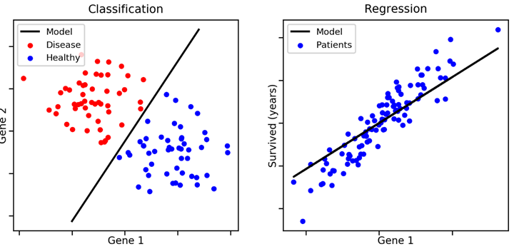
Supervised Learning
- Goal
- Given data $X$ in feature sapce and the labels $Y$
- Learn to predict $Y$ from $X$
- Labels could be discrete or continuous
- Continuous-valued labels: Regression
- Discrete-valued labels: Classification - I don't care
Notation
In this lecture, we will use
- Data $x \in \mathbb{R}^D$ (scalar- or vector-valued)
- Features $\phi(x) \in \mathbb{R}^M$ for data $x$
- Continuous-valued labels $t \in \mathbb{R}$ (target values)
We will use
- $x^{(n)}$ to denote the $n^\text{th}$ training example.
- $t^{(n)}$ to denote the $n^\text{th}$ target value.
Linear Regression (1d inputs)
- Consider 1d case (e.g. D=1)
- Given a set of observations $x^{(1)}, \dots, x^{(N)}$
- and corresponding target values $t^{(1)}, \dots, t^{(N)}$
- We want to learn a function $y(x, {w}) \approx t$ to predict future values.
$$ y(x, {w}) = w_0 + w_1 x + w_2 x^2 + \dots w_M x^M = \sum_{k=0}^M w_k x^k $$
Regression: Noisy Data
xx, yy = generateData(100, False)  # Truth, without noise
x, y = generateData(13, True)      # Noisy observation, training samples
plt.plot(xx, yy, 'g--')
plt.plot(x, y, 'ro');

Regression: 0th Order Polynomial
coeffs = np.polyfit(x, y, 0)  # Leveraging NumPy's polyfit as short-cut; 0 is the degree of the poly
poly = np.poly1d(coeffs) # Polynomial with "learned" parameters
plt.plot(xx, yy, "g--")
plt.plot(x, y, "ro")
plt.plot(xx, poly(xx), "b-");

Regression: 1st Order Polynomial
coeffs = np.polyfit(x, y, 1) # Now let's try degree = 1
poly = np.poly1d(coeffs)
plt.plot(xx, yy, "g--")
plt.plot(x, y, "ro")
plt.plot(xx, poly(xx), "b-");

Regression: 3rd Order Polynomial
coeffs = np.polyfit(x, y, 3) # Now degree = 3
poly = np.poly1d(coeffs)
plt.plot(xx, yy, "g--")
plt.plot(x, y, "ro")
plt.plot(xx, poly(xx), "b-");

Linear Regression (General Case)
The function $y({x}, {w})$ is linear in parameters ${w}$.
- Goal: Find the best value for the weights, ${w}$.
- For simplicity, add a bias term $\phi_0({x}) = 1$.
$$ y({x}, {w}) = w_0 + \sum_{j=0}^{M-1} w_j \phi_j({x}) = {w}^T \phi({x}) $$
Basis Functions
The basis functions $\phi_j({x})$ need not be linear.
r = np.linspace(-1,1,100)
f, axs = plt.subplots(1, 3, figsize=(12,4))
for j in range(8):
    axs[0].plot(r, np.power(r,j))
    axs[1].plot(r, np.exp( - (r - j/7.0 + 0.5)**2 / 2*5**2 ))
    axs[2].plot(r, 1 / (1 + np.exp( - (r - j/5.0 + 0.5) * 5)) )

set_nice_plot_labels(axs)

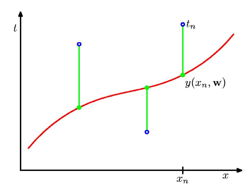
Least Squares: Objective Function
Minimize the residual error over the training data.
$$ E({w}) = \frac12 \sum_{n=1}^N (y(x^{(n)}, {w}) - t^{(n)})^2 = \frac12 \sum_{n=1}^N \left( \sum_{j=0}^{M-1} w_j\phi_j({x}^{(n)}) - t^{(n)} \right)^2 $$
Least Squares: Gradient Calculation
Closed Form Solution: Derivation
$$ \begin{aligned} \text{Scalar Form: } E({w}) &= \frac12 \sum_{n=1}^N \left( \sum_{j=0}^{M-1} w_j \phi_j({x}^{(n)}) - t^{(n)} \right)^2 \\ &= \frac12 \sum_{n=1}^N \left( {w}^T \phi({x}^n) - t^{(n)} \right)^2 \\ &= \frac12 \sum_{n=1}^N ({w}^T \phi( {x}^{(n)} ) )^2 - \sum_{n=1}^N t^{(n)} {w}^T \phi( {x}^{(n)} ) + \frac12 \sum_{n=1}^N (t^{(n)})^2 \\ \mbox{Vector Form: } E({w}) &= \frac12 \|\Phi {w} - {t}\|^2 \\ &= \frac12 {w}^T \Phi^T \Phi {w} - {w}^T \Phi^T {t} + \frac12 {t}^T {t} \end{aligned} $$
Closed Form Solution: Data Matrix
The design matrix is a matrix $\Phi \in \mathbb{R}^{N \times M}$, applying
- the $M$ basis functions (columns)
- to $N$ data points (rows)
$$ \Phi = \begin{bmatrix} \phi_0({x}^{(1)}) & \phi_1({x}^{(1)}) & \cdots & \phi_{M-1}({x}^{(1)}) \\ \phi_0({x}^{(2)}) & \phi_1({x}^{(2)}) & \cdots & \phi_{M-1}({x}^{(2)}) \\ \vdots & \vdots & \ddots & \vdots \\ \phi_0({x}^{(N)}) & \phi_1({x}^{(N)}) & \cdots & \phi_{M-1}({x}^{(N)}) \\ \end{bmatrix} $$
Goal: $\Phi {w} \approx {t}$
Least Squares: Gradient via Matrix Calculus
- Compute the gradient and set to zero
$$ \begin{aligned} \nabla_{w} E({w}) &= \nabla_{w} \left[ \frac12 {w}^T \Phi^T \Phi {w} - {w}^T \Phi^T {t} + \frac12 {t}^T {t} \right] \\ &= \Phi^T \Phi {w} - \Phi^T {t} = 0 \end{aligned} $$
- Solve the resulting normal equation: $$ \Phi^T \Phi {w} = \Phi^T {t},\quad {w} = (\Phi^T \Phi)^{-1} \Phi^T {t} $$
This is the Moore-Penrose pseudoinverse, $\Phi^\dagger = (\Phi^T \Phi)^{-1} \Phi^T$ applied to solve the linear system $\Phi {w} \approx {t}$.
Digression: Moore-Penrose Pseudoinverse
- When we have a matrix $A$ that is non-invertible or not even square, we might want to invert anyway
- For these situations we use $A^\dagger$, the Moore-Penrose Pseudoinverse of $A$
- When $A$ has lin. indep. columns then $A^\dagger = (A^\top A)^{-1} A^\top$
- In general, we can get $A^\dagger$ by SVD: if we write $A = U \Sigma V^\top$ then $A^\dagger = V \Sigma^\dagger U^\top$, where $\Sigma^\dagger$ is obtained by taking reciprocals of non-zero entries of $\Sigma$.
Alternative View: Projection onto subspace
- Columns of $\Phi$ forms a subspace and we are essentially projecting ${t}$ onto $\Phi$ when doing $\Phi {x}={t}$
- The SVD $\Phi=U\Sigma V^T$ produces the orthonormal basis $U$ and transformation matrix $T=\Sigma V^T$
- Recall from review of linear algebra, let ${y}=T{x}$, then $U{y}={t}$ and ${y}\approx U^T{t}$
- Then ${x}=T^{-1}{y}=V\Sigma^\dagger U^T {t}=\Phi^\dagger {t}$
Detailed derivation - Scalar version - Skip in class
Least Squares: Gradient Calculation
To minimize the error, take partial derivatives w.r.t. each weight $w_j$:
$$ \frac{\partial E({w})}{\partial w_k}= \frac{\partial}{\partial w_k} \left[ \frac12 \sum_{n=1}^N \left( \sum_{j=0}^{M-1} w_j\phi_j({x}^{(n)}) - t^{(n)} \right)^2 \right] $$
Apply the chain rule:
$$ = \sum_{n=1}^N \left[ \left( \sum_{j=0}^{M-1} w_j\phi_j({x}^{(n)}) - t^{(n)} \right) \frac{\partial}{\partial w_k} \left[ \sum_{j=0}^{M-1} w_j\phi_j({x}^{(n)}) - t^{(n)} \right] \right] $$
$$ = \sum_{n=1}^N \left[ \left( \sum_{j=0}^{M-1} w_j\phi_j({x}^{(n)}) - t^{(n)} \right) \phi_k({x}^{(n)}) \right] $$
Least Squares: Vectorized Gradient
$$ \begin{aligned} \nabla_w E({w}) &= \sum_{n=1}^N \left( \sum_{j=0}^{M-1} w_j \phi_j({x}^{(n)}) - t^{(n)} \right) \phi({x}^{(n)}) \\ &= \sum_{n=1}^N \left( {w}^T \phi({x}^{(n)}) - t^{(n)} \right) \phi({x}^{(n)}) \end{aligned} $$
Closed Form Solution
Main Idea: Compute gradient and set to gradient to zero, solving in closed form.
- Objective function: $$E({w}) = \frac12 \sum_{n=1}^N \left( \sum_{j=0}^{M-1} w_j\phi_j({x}^{(n)})- t^{(n)}\right)^2$$
- We will derive the gradient using matrix calculus.
Detailed derivation - Matrix Calculus - Skip in class
Matrix Calculus: The Gradient
Suppose that $f : \mathbb{R}^{m \times n} \mapsto \mathbb{R}$, that is, the function $f$
- takes as input a matrix $A \in \mathbb{R}^{m\times n} = [a_{ij}]$
- returns a real value
Then, the gradient of $f$ with respect to $A$ is:
$$ \nabla_A f(A) \in \mathbb{R}^{m \times n} = \begin{bmatrix} % \frac{\partial f}{\partial a_{11}} & \frac{\partial f}{\partial a_{12}} & \cdots & \frac{\partial f}{\partial a_{1n}} \\ % \frac{\partial f}{\partial a_{21}} & \frac{\partial f}{\partial a_{22}} & \cdots & \frac{\partial f}{\partial a_{2n}} \\ % \vdots & \vdots & \ddots & \vdots \\ % \frac{\partial f}{\partial a_{m1}} & \frac{\partial f}{\partial a_{m2}} & \cdots & \frac{\partial f}{\partial a_{mn}} \\ \end{bmatrix},\quad [\nabla_A f(A)]_{ij} = \frac{\partial f}{\partial a_{ij}} $$
Matrix Calculus: The Gradient
Note that the size of $\nabla_A f(A)$ is always the same as the size of $A$. In particular, for vectors $x \in \mathbb{R}^n$,
$$ \nabla_x f(x) = \begin{bmatrix} \frac{\partial f}{\partial x_1} & \frac{\partial f}{\partial x_2} & \cdots & \frac{\partial f}{\partial x_n} \end{bmatrix}^T $$
The gradient is a linear operator from $\mathbb{R}^n \mapsto \mathbb{R}^n$:
- $ \nabla_x (f + g) = \nabla_x f + \nabla_x g $
- $ \forall\, c \in R, \nabla_x (c f) = c \nabla_x f$
Gradient: Linear Functions
The gradient of the linear function $f(x) = \sum_{k=1}^n b_k x_k = b^T x$ is
$$ \frac{\partial f}{\partial x_k} = \frac{\partial}{\partial x_k} \sum_{k=1}^n b_k x_k = \sum_{k=1}^n \frac{\partial}{\partial x_k} b_k x_k = b_k $$
In a more compact form,
$$ \nabla_x b^T x = b $$
Gradient: Quadratic Forms
- Every symmetric $A \in \mathbb{R}^{n \times n}$ corresponds to a quadratic form: $$ f(x) = \sum_{i=1}^n \sum_{j=1}^n x_i A_{ij} x_j = x^T A x $$
- The partial derivatives are $$ \frac{\partial f}{\partial x_k} = 2 \sum_{j=1}^n A_{ij} x_j = 2 [Ax]_i $$
- Compact form $\nabla_x f(x) = 2 Ax$
stys = ['k-', 'k-.', 'm-', 'm-.']
plt.plot(xx, yy, "g--")
plt.plot(x, y, "ro", label="Training data")
for _i in range(4):
    plt.plot(xx, tsts[_i], stys[_i], label='Order {0}'.format(_i))
plt.legend();

Root of Mean-Squared Error, RMSE
$$ E_{RMS} = \sqrt{2E(w^*) / N} = \sqrt{\frac{1}{N}\sum_{i=1}^N[f(x^{(i)})-t^{(i)}]^2} $$
- Easy to compute
- Potential issue: Improperly scaled
f, ax = plt.subplots(ncols=4, sharey=True, figsize=(16,4))
for _i in range(4):
    ax[_i].plot(xx, yy, "g--")
    ax[_i].plot(x, y, "ro")
    ax[_i].plot(xx, tsts[_i])
    ax[_i].set_title('Order {0}, RMSE={1:4.3f}'.format(_i, es[_i]))

Coefficient of determination
$$ R^2 = 1 - \frac{SS_{res}}{SS_{tot}} $$
- Let $\bar{t}$ be average of $\{t_i\}$
- Residual sum of squares: $$SS_{res}=\sum_i[f(x^{(i)})-t^{(i)}]^2$$
- Total sum of squares: $$SS_{tot}=\sum_i[t^{(i)}-\bar{t}]^2$$
- Explained sum of squares: $$SS_{reg}=\sum_i[f(x^{(i)})-\bar{t}]^2$$
- In simple least squares: $$SS_{tot}=SS_{reg}+SS_{res}$$
f, ax = plt.subplots(ncols=4, sharey=True, figsize=(16,4))
for _i in range(4):
    ax[_i].plot(y, y, "r-")
    ax[_i].plot(y, trns[_i], "bo")
    ax[_i].set_title('Order {0}, R2={1:4.3f}'.format(_i, rs[_i]))

Geometrical interpretation of R2
- Blue: Squared residuals w.r.t. the linear regression.
- Red: Squared residuals w.r.t. the average value.
$$ R^2 = 1 - \frac{\color{blue}{SS_{res}}}{\color{red}{SS_{tot}}} $$
