Machine Learning for Engineering

Linear Regression: Model Selection

Instructor: Daning Huang

TODAY: Linear Regression - IV

• Bias-variance tradeoff
• Methods for model selection
  • Cross validation
  • Information criteria

References:

• [PRML] Chps. 3.2-3.5
• [MLaPP] Chp. 5.3, 6.4

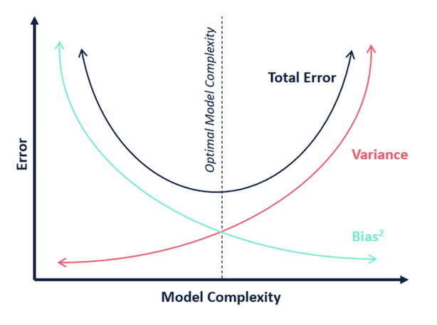
Bias-Variance Tradeoff

Bias and Variance Formulae

• Consider $y(x) = f^*(x) + \epsilon$
  • $f^*$ is the true model
  • $\epsilon$ is some $0$-mean noise with variance $\sigma^2$
• A model receives one dataset $S$ and outputs $\hat f$ as prediction of $y$. The error is:

$$\mathbb{E}[(y - \hat{f})^2] = \underbrace{{\sigma^2}}_\text{irreducible error} + \underbrace{{\text{Var}[\hat{f}]}}_\text{Variance} + \underbrace{(f - \mathbb{E}[\hat{f}])^2}_{\text{Bias}^2}$$

where expectation is taken w.r.t. all possible datasets, $\mathbb{E}[f(S)]=\mathbb{E}_S[f(S)]=\int f(S)p(S)dS$.

• Break error into two terms relating to $\mathbb{E}[\hat f]$ the "average" estimate over random datasets $S$.
  • Irreducible error: Minimum possible error - determined by measurement noise
  • Bias: Fitting capability - "complexity" of model
  • Variance: Generalization capability - Model sensitivity to changes in dataset, (overfitting)

An example to explain Bias/Variance and illustrate the tradeoff

• Consider estimating a sinusoidal function.

(Example that follows is inspired by Yaser Abu-Mostafa's CS 156 Lecture titled "Bias-Variance Tradeoff"

Let's return to fitting polynomials

• Here we generate some samples $x,y$, with $y = \sin(\pi x)$
• We then fit a degree-$0$ polynomial (i.e. a constant function) to the samples

# polyfit_sin() generates 5 samples of the form (x,y) where y=sin(pi*x)
# then it tries to fit a degree=0 polynomial (i.e. a constant func.) to the data
# Ignore return values for now, we will return to these later
_, _, _, _ = polyfit_sin(degree=0, iterations=1, num_points=5, show=True)

We can do this over many datasets

• Let's sample a number of datasets
• How does the fitted polynomial change for different datasets?

# Estimate two points of sin(pi * x) with a constant 5 times
_, _, _, _ = polyfit_sin(degree=0, iterations=5)

What about over lots more datasets?

# Estimate two points of sin(pi * x) with a constant 100 times
_, _, _, _ = polyfit_sin(degree=0, iterations=100)

MSE, errs, mean_coeffs, coeffs_list = polyfit_sin(degree=0, iterations=100, num_points=3, show=False)
biases, variances = calculate_bias_variance(coeffs_list,RANGEXS,TRUEYS)
plot_bias_and_variance(biases,variances,RANGEXS,TRUEYS,np.polyval(np.poly1d(mean_coeffs), RANGEXS))

• Decomposition: $\mathbb{E}[(y - \hat{f})^2] = \underbrace{{\sigma^2}}_\text{irreducible error} + \underbrace{{\text{Var}[\hat{f}]}}_\text{Variance} + \underbrace{(f - \mathbb{E}[\hat{f}])^2}_{\text{Bias}^2}$
• Blue curve: true $f$
• Black curve: $\hat f$, average predicted values of $y$
• Yellow is error due to Bias, Red/Pink is error due to Variance

Bias vs. Variance

• We can calculate how much error we suffered due to bias and due to variance

poly_degree, results_list = 0, []
MSE, errs, mean_coeffs, coeffs_list = polyfit_sin(poly_degree, 500,num_points = 5,show=False)
biases, variances = calculate_bias_variance(coeffs_list,RANGEXS,TRUEYS)
sns.barplot(x='type', y='error',hue='poly_degree', data=pd.DataFrame([{'error':np.mean(biases), 'type':'bias','poly_degree':0},
    {'error':np.mean(variances), 'type':'variance','poly_degree':0}]))

<AxesSubplot:xlabel='type', ylabel='error'>

Let's now fit degree=3 polynomials

• Let's sample a dataset of 5 points and fit a cubic poly

MSE, _, _, _ = polyfit_sin(degree=3, iterations=1)

Let's now fit degree=3 polynomials

• What does this look like over 5 different datasets?

_, _, _, _ = polyfit_sin(degree=3,iterations=5,num_points=5,show=True)

Let's now fit degree=3 polynomials

• What does this look like over 50 different datasets?

# Estimate two points of sin(pi * x) with a line 50 times
_, _, _, _ = polyfit_sin(degree=3, iterations=50)

MSE, errs, mean_coeffs, coeffs_list = polyfit_sin(3,500,show=False)
biases, variances = calculate_bias_variance(coeffs_list,RANGEXS,TRUEYS)
plot_bias_and_variance(biases,variances,RANGEXS,TRUEYS,np.polyval(np.poly1d(mean_coeffs), RANGEXS))

$$\mathbb{E}[(y - \hat{f})^2] = \underbrace{{\sigma^2}}_\text{irreducible error} + \underbrace{{\text{Var}[\hat{f}]}}_\text{Variance} + \underbrace{(f - \mathbb{E}[\hat{f}])^2}_{\text{Bias}^2}$$

• Blue curve: true $f$
• Black curve: $\mathbb{E}[\hat f]$, average prediction of $y$
• Yellow is error due to Bias, Red/Pink is error due to Variance

Bias and Variance for different degree sizes

sns.barplot(x='type', y='error',hue='poly_degree',data=pd.DataFrame(results_list));

<AxesSubplot:xlabel='type', ylabel='error'>

• High degree polys have lower bias but much greater variance!
• Bias-Variance Trade-off

Examples - Linear Regression

Consider $m$ features $\phi(x)$ and $n$ data points of noise level $\sigma^2$.

The trade-off is approximately (very crude!) $$ \mathbb{E}[(y - \hat{f})^2] = \underbrace{O({\sigma^2})}_\text{irreducible error} + \underbrace{O(\sigma^2\frac{m}{n})}_\text{Variance} + \underbrace{O(m^{-p})}_{\text{Bias}^2} $$

• Variance: $m$ competes with $n$.
• Bias reduces as $m$ increases.

Examples - Ridge Regression

Adding the regularization factor $\lambda$, the trade-off is modified with an effective number of features $$ \mathbb{E}[(y - \hat{f})^2] = \underbrace{O({\sigma^2})}_\text{irreducible error} + \underbrace{O(\sigma^2\frac{{\tilde{m}}}{n})}_\text{Variance} + \underbrace{O({\tilde{m}}^{-p})}_{\text{Bias}^2} $$ where $$ {\tilde{m}} = \sum_{j=1}^m \frac{\nu_i}{\nu_i+\lambda} $$ and $\nu_i$'s are the eigenvalues of $\Phi^\top\Phi$.

• For $\lambda>0$, ${\tilde{m}}<m$ - effectively reduces model complexity.
• When $\lambda=0$, ${\tilde{m}}=m$ and simple linear regression is recovered.
• When $\lambda\rightarrow\infty$, ${\tilde{m}}\rightarrow 0$ and we get a naive model (always predicts 0).

For more precise expressions and more challenging cases such as Lasso, see this note.

Methods for Model Selection

Choosing the model with the right complexity

• e.g. choose $\alpha$ in Ridge Regression, see [PRML] Chp. 3.5 for more details

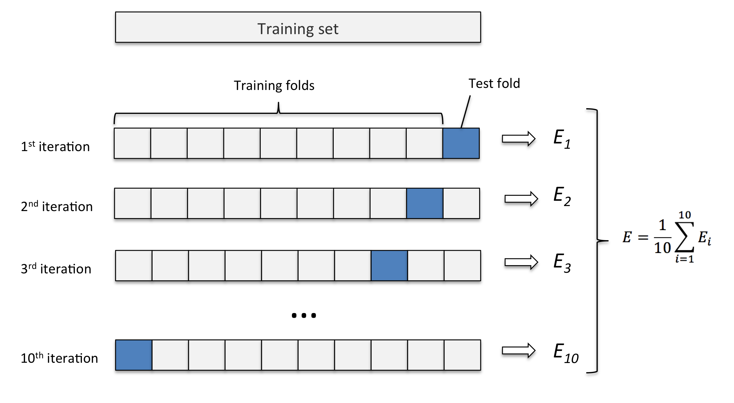
Cross-Validation

For a model $M(\alpha)$ with complexity parameter $\alpha$

• Split the dataset into K-fold
• For i=1,...,K
  • Remove the ith fold and train a model
  • Compute the error $E_i$ on the ith fold
• Average all the errors $E_1$,...,$E_K$ to obtain the estimated error of $M(\alpha)$

Repeat for different $\alpha$'s and find the one with minimum error

• Leave-One-Out (LOO): Divide a dataset having N samples into N-fold
• Advantages:
  • Good when not many samples are available (otherwise one can create datasets for training and validation)
  • Attenuates impact of overfitting - trying out many possible combinations of datasets
• Disadvantages:
  • Computationally expensive - K-fold CV requires training the model K times
  • Inconvenient if the model has multiple complexity parameters - Grid-search? Could be expensive

Information criteria

• Akaike information criteria (AIC) $$ AIC = 2M - 2\ln p(t|w_{ML}) $$
• Bayesian information criteria (BIC) $$ BIC = M\ln N - 2\ln p(t|w_{MAP}) $$
• $M$: number of complexity parameters, $N$: number of samples
• For linear regression: $$ \begin{align} -2\ln p(t|w) &= -N \ln\beta + N \ln{2\pi} + 2\beta E_D(w) \\ &= N\ln\frac{E_D(w)}{N} + const \end{align} $$

• Both are easy to evaluate - but not straightforward for interpretation
• BIC penalizes more on model complexity than AIC
• BIC works better when $N\gg M$

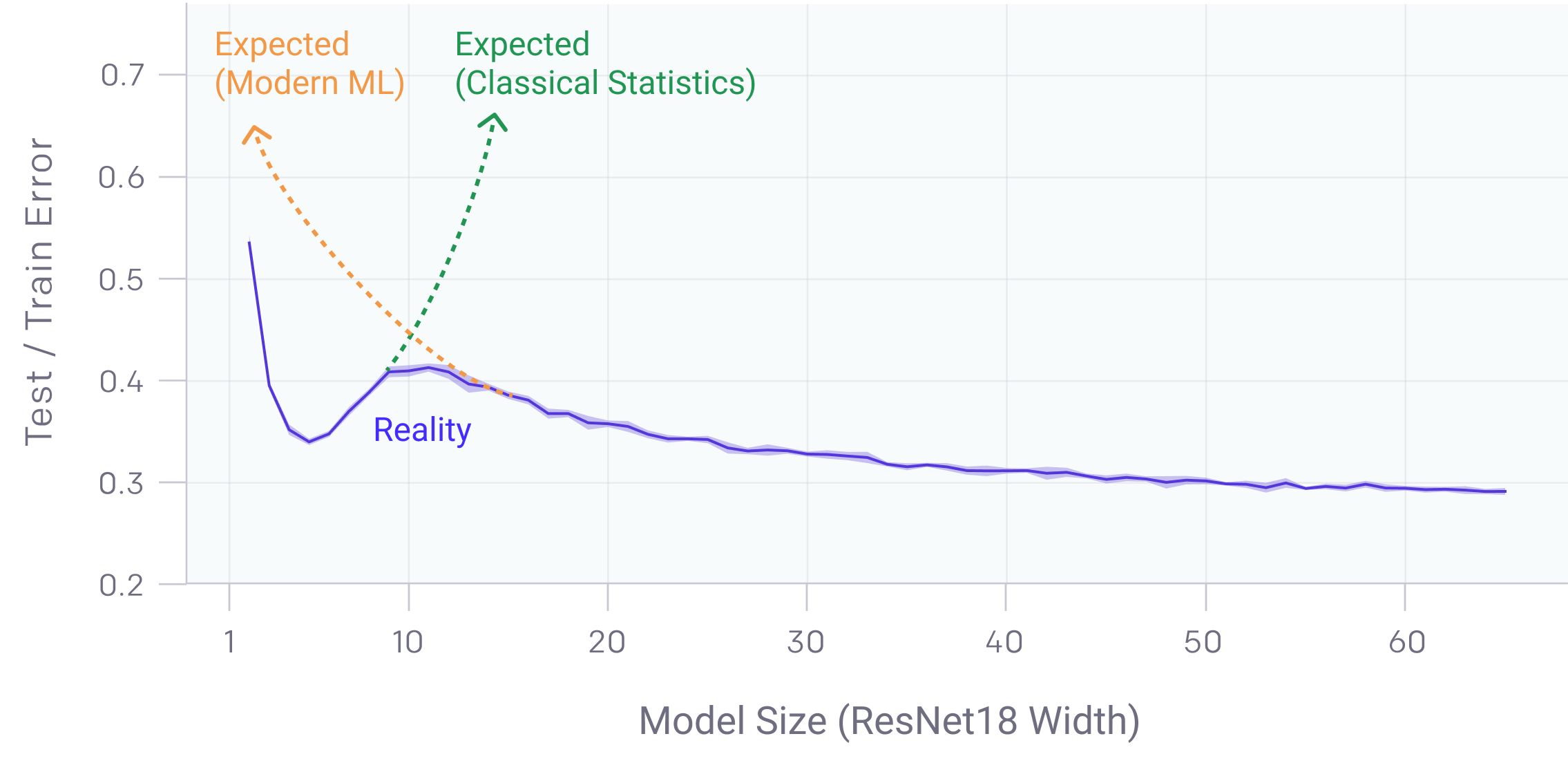
Deep Double Descent in Over-parametrized Case

AKA in deep learning: https://openai.com/blog/deep-double-descent/

A simple experiment: Consider a quantity $y$ and its measurements (i.e. features) $x_1,x_2,\cdots,x_F$

• The first $K$ features are $x_i=z_i+y$, where $z_i$ is unit Gaussian noise
• The latter $F-K$ features are merely noise, $x_i=z_i$

We will fit a series of models for $y$ using 100 samples with increasing number of features $M$.

• When $M\leq 100$, regular least squares suffices;
• When $M>100$ least norm squares is needed (but pseudo inverse just works fine).

Intuition:

• The first $K$ features carry information about $y$ - so the more of these features are used, the better is the prediction
• The rest $M-K$ features should not improve the prediction

But is this the case?

f = plt.figure(figsize=(6,4))
plt.plot(nins, ets, 'b-', label='Training')
plt.plot(nins, ess, 'r-', label='Test')
plt.plot([nfea, nfea], [0,1], 'k--')
plt.legend()
plt.ylim([0,1])
plt.xlabel('# of features')
plt.ylabel('Average error')

Text(0, 0.5, 'Average error')

In fact, beyond the Bias-Variance curve, the test error still drops, after a short increase.

• For this particular problem, the extra features help cancel out the noise in the "useful" features.
• Still an open question for deep learning community...