MLE & MAP
Maximum Likelihood: Pick the parameters under which the data is most probable under our model.
$$ w_{ML} = \arg\max_w P(\mathcal{X} | w) $$
Maximum a Posteriori: Pick the parameters under which the data is most probable, weighted by our prior beliefs.
$$ w_{MAP} = \arg\max_w P(\mathcal{X} | w) P(w) $$
Maximum Likelihood Interpretation of Least Squares Regression
Maximum Likelihood $w$
Assume a stochastic model $$ \begin{gather} t = y(x,w) + \epsilon \\ \epsilon \sim \mathcal{N}(0, \beta^{-1}) \end{gather} $$ where $\beta$ represents precision.
This gives the following likelihood function: $$ p(t|x,w,\beta) = \mathcal{N}(t|y(x,w),\beta^{-1}) $$
Maximum Likelihood $w$
- With inputs $X=(x_1, \dots, x_n)$ and target values $t=(t_1,\dots,t_n)$, the data likelihood is $$ p(t|X,w,\beta) = \prod_{n=1}^N \mathcal{N}(t_n|w^T\phi(x_n),\beta^{-1}) $$
For conciseness, now we use $\Box_n$ to denote the $n$th sample, instead of $\Box^{(n)}$
Log Likelihood
We will now show that the log likelihood is $$ \ln p(t|X,w,\beta) = \frac{N}{2} \ln\beta - \frac{N}{2} \ln{2\pi}- \beta E_D(w) $$ where $$ E_D(w) = \frac{1}{2} \sum_{n=1}^N \left[ t_n-w^T\phi(x_n) \right]^2 = \frac{1}{2} \|t-\Phi w\|^2 $$
Recall the design matrix $\Phi$: $$ \Phi = \begin{bmatrix} \phi_0({x}_1) & \phi_1({x}_1) & \cdots & \phi_{M-1}({x}_1) \\ \phi_0({x}_2) & \phi_1({x}_2) & \cdots & \phi_{M-1}({x}_2) \\ \vdots & \vdots & \ddots & \vdots \\ \phi_0({x}_N) & \phi_1({x}_N) & \cdots & \phi_{M-1}({x}_N) \\ \end{bmatrix} $$
Details of Derivation - 1/2
From $P(t| x,w) = \sqrt\frac{\beta}{2\pi} \exp(-\frac{\beta}{2} \| t-w^T \phi(x) \|^2)$ we have $$ \begin{aligned} &\; \ln P(t_1, \dots, t_N | x,w) \\ =&\; \ln \prod_{k=1}^N \mathcal{N}(t_k| w^T \phi(x^{(k)}), \beta^{-1}) \\ =& \sum_{k=1}^N \ln \left[ \sqrt\frac{\beta}{2\pi} \exp \left( -\frac{\beta}{2} \| t_k-w^T \phi(x^{(k)}) \|^2 \right) \right] \end{aligned} $$
Details of Derivation - 2/2
$$ \begin{aligned} =&\; \sum_{k=1}^N \ln \left[ \sqrt\frac{\beta}{2\pi} \exp(-\frac{\beta}{2} ( t_k-w^T \phi(x^{(k)}) )^2) \right] \\ =&\; \sum_{k=1}^N \left[ \frac{1}{2} \ln\beta - \frac{1}{2}\ln{2\pi} - \frac{\beta}{2}( t_k - w^T\phi(x_k) )^2 \right] \\ =&\; \frac{N}{2} \ln\beta - \frac{N}{2} \ln{2\pi} - \beta \sum_{k=1}^N \frac{1}{2}( t_k - w^T\phi(x_k) )^2 \\ \end{aligned} $$
Maximize the Likelihood
Maximizing the likelihood is equivalent to minimizing the sum of squared errors
Set gradient of log-likelihood to zero, $$ \begin{aligned} \nabla_w \ln p(t | w, \beta) &= \nabla_w \left[ \frac{N}{2}\ln\beta - \frac{N}{2}\ln{2\pi} - \beta E_D(w) \right] = 0 \\ &\Rightarrow \beta\nabla_w \left[ \frac{1}{2} \|t-\Phi w\|^2 \right] = 0 \\ &\Rightarrow \boxed{(\Phi^T \Phi) w = \Phi^T t} \end{aligned} $$
Scalar version of derivation - Skip in class
$$ \begin{aligned} \nabla_w \ln p(t | w, \beta) &= \nabla_w \left[ \frac{N}{2}\ln\beta - \frac{N}{2}\ln{2\pi} - \beta \sum_{n=1}^N \frac{1}{2} \left( t_n - w^T \phi(x_n) \right)^2 \right] = 0 \\ &\Rightarrow \nabla_w \left[ - \beta \sum_{n=1}^N \frac{1}{2} \left( t_n - w^T \phi(x_n) \right)^2 \right] \\ &= \beta \sum_{n=1}^N \nabla_w \left[ -\frac{1}{2} \left( t_n - w^T \phi(x_n) \right)^2 \right] \\ &= \beta \sum_{n=1}^N \left[ t_n - w^T \phi(x_n) \right] \phi(x_n)^T = 0 \\ &\Rightarrow \sum_{n=1}^N \left[ t_n - w^T \phi(x_n) \right] \phi(x_n)^T = 0 \\ 0 &= \sum_{n=1}^N t_n \phi(x_n)^T - w^T \left[ \sum_{n=1}^N \phi(x_n) \phi(x_n)^T \right] \end{aligned} $$
- Similarly, one can determine $\beta$, i.e. the precision of the prediction, $$ \begin{aligned} \nabla_\beta \ln p(t | w, \beta) &= \nabla_\beta \left[ \frac{N}{2}\ln\beta - \frac{N}{2}\ln{2\pi} - \beta E_D(w) \right] = 0 \\ &\Rightarrow \frac{N}{2\beta} - \sum_{n=1}^N \frac{1}{2} \left[ t_n - w^T \phi(x_n) \right]^2 = 0 \\ &\Rightarrow \beta^{-1} = \frac{1}{N}\sum_{n=1}^N \left[ t_n - w^T \phi(x_n) \right]^2 = \frac{E_D(w)}{N} \end{aligned} $$
- Eventually we get a predictive distribution $$ p(t|x,w,\beta) = \mathcal{N}(t|w^T\phi(x),\beta^{-1}) $$
- This formulation provides an estimation of precision
Maximum a posteriori Interpretation of Regularized Regression
Problem setup
Again we assume a stochastic model $$ \begin{aligned} t &= y(x,w) + \epsilon \\ \epsilon &\sim \mathcal{N}(0, \beta^{-1}) \end{aligned} $$ where $\beta$ represents accuracy.
With inputs $X=(x_1, \dots, x_n)$ and target values $t=(t_1,\dots,t_n)$, the data likelihood is $$ p(t|w,\beta) = \prod_{n=1}^N \mathcal{N}(t_n|w^T\phi(x_n),\beta^{-1}) $$ (Note $X$ is omitted for simplicity)
- But this time we add a prior on $w$, representing what we "believe" $w$ should be like.
- For example, a Gaussian prior $$ p(w|\alpha) = \mathcal{N}(0, \alpha^{-1}I) $$ means $w$ should be centered around zero, i.e. unlikely to have large values.
- In general a multivariate Gaussian is $$ \mathcal{N}(\mu, \Sigma) = \frac{1}{\sqrt{(2\pi)^k|\Sigma|}} \exp \left[ -\frac{1}{2}(x-\mu)^T\Sigma^{-1}(x-\mu)) \right] $$ where $\mu\in\mathbb{R}^k$, $\Sigma\in\mathbb{R}^{k\times k}$
MAP estimation
- Given the likelihood and the prior, using Bayes' rule, $$ p(w|t,\alpha,\beta) \propto p(t|w,\beta)p(w|\alpha) $$
- Taking the logarithm again, $$ \begin{aligned} \ln p(w|t,\alpha,\beta) &= \color{red}{\ln p(t|w,\beta)} + \color{blue}{\ln p(w|\alpha)} + const \\ &= \color{red}{\frac{N}{2} \ln\beta - \frac{\beta}{2} \sum_{k=1}^N ( t_k - w^T\phi(x_k) )^2} \color{blue}{- \frac{\alpha}{2} ||w||^2} + const \end{aligned} $$
- Looking familiar? Essentially the regularized objective function from optimization approach $$ \color{red}{E_D(w)}+\lambda \color{blue}{E_W(w)},\quad \lambda=\frac{\alpha}{\beta} $$
- The posterior $p(w|t,\alpha,\beta)$ turns out to be Gaussian too, and $$ p(w|t,\alpha,\beta) = \mathcal{N}(m_N,S_N) $$ where $m_N$ is the estimated parameter, and $S_N$ is the precision, $$ \begin{aligned} m_N &= \beta S_N \Phi^T t \\ S_N^{-1} &= \alpha I + \beta \Phi^T\Phi \end{aligned} $$
- [Gaussian Identity I] Above result is due to a nice property of Gaussian distribution: If the likelihood and prior are Gaussian, then the posterior is Gaussian
$$
\begin{aligned}
p(x) &= \mathcal{N}(x|\mu,\Lambda^{-1}) \\
p(y|x) &= \mathcal{N}(y|Ax+b,L^{-1}) \\
\Rightarrow p(x|y) &= \mathcal{N}(x|\Sigma[A^TL(y-b)+\Lambda\mu],\Sigma)
\end{aligned}
$$
where $\Sigma=(\Lambda + A^TLA)^{-1}$.
- Further explanation: See extra material on the exponential family
Predictive distribution
- We care about predicting $t$ more than estimating $w$.
- The predictive distribution of $t$ is given by a marginalization $$ p(t_i|t,\alpha,\beta) = \int p(t_i,w|t,\alpha,\beta)dw = \int p(t_i|w,\beta)p(w|t,\alpha,\beta) dw $$
- It turns out $$ p(t_i|x,t,\alpha,\beta) = \mathcal{N}(t_i|m_N^T\phi(x), \sigma_N^2(x)) $$ where $$ \sigma_N^2(x) = \frac{1}{\beta} + \phi(x)^T S_N \phi(x) $$
- [Gaussian Identity II] Above result is due to another nice property of Gaussian distribution: $$ \begin{aligned} p(x) &= \mathcal{N}(x|\mu,\Lambda^{-1}) \\ p(y|x) &= \mathcal{N}(y|Ax+b,L^{-1}) \\ \Rightarrow p(y) &= \mathcal{N}(y|A\mu+b,L^{-1}+A\Lambda^{-1}A^T) \end{aligned} $$
- The Bayesian approach provides the error estimate of the ridge regression, something missing from the optimization approach.
Visualization - Linear curve fitting example
$$ y=\underbrace{0.5}_{w_1}+\underbrace{2}_{w_2}x+\epsilon $$
- Left: Distributions of the weights $w$
- Right: Samples of the linear fit
There are many knobs in this example:
- Initial setup: $\epsilon\sim10^{-6}$, $\alpha=10^{-6}$, $\beta=1$
- Increase number of samples from 0 to 100
- Observe the changes in weight space and the predictive variance.
- Keeping 10 samples
- Confidence in data: Vary $\beta$ from $10^2$ to $10^{-6}$
- Confidence in prior: Vary $\alpha$ from $10^2$ to $10^{-6}$
- Data quality: Vary noise level from $10^{-6}$ to $1$
N = 1  # Only 1 data point
x, t = xSmpl[:N], tSmpl[:N]
mN, SN = pwD(x, t, alpha, beta); print(mN)

f, ax = plt.subplots(ncols=2, figsize=(16,8))
pltMvN(ax[0], mN, SN)
pltSmp(ax[1], x, t, mN, SN, beta, bnd=True)
[1.0627721 0.52247489]

N = 2  # Increase to 2 data points
x, t = xSmpl[:N], tSmpl[:N]
mN, SN = pwD(x, t, alpha, beta); print(mN)

f, ax = plt.subplots(ncols=2, figsize=(16,8))
pltMvN(ax[0], mN, SN)
pltSmp(ax[1], x, t, mN, SN, beta, bnd=True)
[0.25215522 2.17136113]

N = 20  # ... and 20 data points
x, t = xSmpl[:N], tSmpl[:N]
mN, SN = pwD(x, t, alpha, beta); print(mN)

f, ax = plt.subplots(ncols=2, figsize=(16,8))
pltMvN(ax[0], mN, SN)
pltSmp(ax[1], x, t, mN, SN, beta, bnd=True)
[0.53079197 1.90442572]

N = 100  # all data points
x, t = xSmpl[:N], tSmpl[:N]
mN, SN = pwD(x, t, alpha, beta); print(mN)

f, ax = plt.subplots(ncols=2, figsize=(16,8))
pltMvN(ax[0], mN, SN)
pltSmp(ax[1], x, t, mN, SN, beta, bnd=True)
[0.51073856 1.97149626]

Visualization - 1
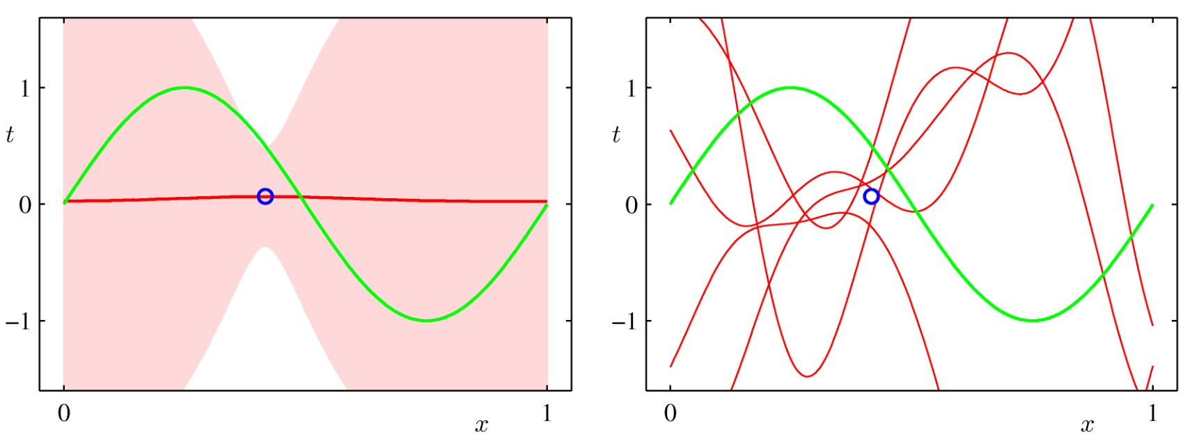
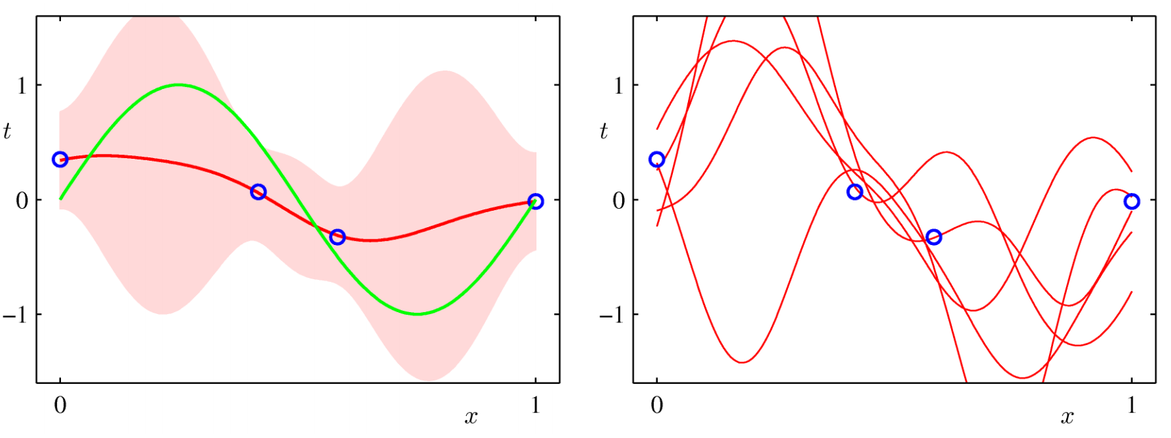
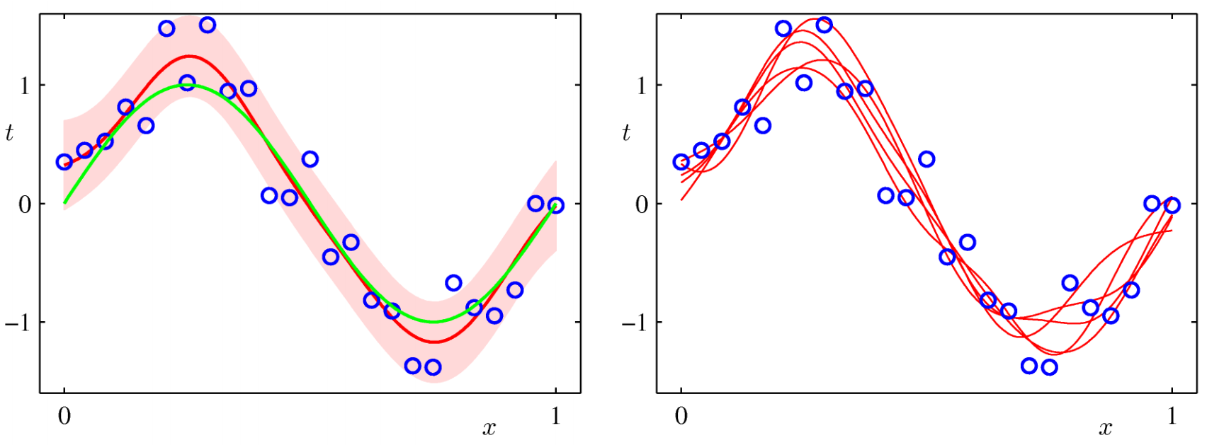
Another example from PRML:
- Green curve: Truth
- Blue dots: Data points
- Red curve: Predictive mean
- Red shade: One standard deviation
- On the right: Samples of $w$
Visualization - 2
Visualization - 3
Determining hyperparameters $\alpha$, $\beta$
- Using Bayes' rule $$ p(\alpha,\beta|t) \propto p(t|\alpha,\beta)p(\alpha,\beta) \approx p(t|\alpha,\beta) $$ assuming $p(\alpha,\beta)$ is relatively "flat"
- So we can find $\alpha$, $\beta$ by maximizing the marginal likelihood function $$ p(t|\alpha, \beta) = \int p(t|w,\beta) p(w|\alpha) dw $$
- Known as Type II maximum likelihood, Evidence approximation, etc.
- After some math we can see that $$ \begin{aligned} \ln p(t|\alpha, \beta) &= \frac{M}{2}\ln\alpha + \frac{N}{2}\ln\beta - E(m_N) - \frac{1}{2}\ln|S_N^{-1}| - \frac{N}{2}\ln(2\pi) \\ E(m_N) &= \frac{\beta}{2}||t-\Phi m_N||^2 + \frac{\alpha}{2}m_N^T m_N \end{aligned} $$
- Setting the gradients of $\ln p(t|\alpha, \beta)$ w.r.t. $\alpha$, $\beta$ to be zero, we can find the re-estimation equations for $\alpha$ and $\beta$ $$ \begin{aligned} \alpha &= \frac{\gamma}{m_N^T m_N},\quad \gamma = \sum_{i=1}^M \frac{\lambda_i}{\alpha+\lambda_i} \\ \beta^{-1} &= \frac{1}{N-\gamma} ||t-\Phi m_N||^2 \end{aligned} $$ where $\lambda_i$ are eigenvalues of $\beta\Phi^T\Phi$
- To the bravest, derive the above results as practice.
- Some observations:
- This is the Bayesian approach to determining the hyperparameters. It is somewhat elegant, but sometimes cumbersome.
- $\gamma$ is considered the effective number of parameters, and now the estimation of $\beta^{-1}$ is unbiased.
- $m_N$ is a function of $\alpha$ and $\beta$ - One would need to iteratively compute $m_N$ and $\alpha$, $\beta$ until convergence.
The iterative procedure to determine $m_N$, $S_N$, $\alpha$, $\beta$
- Guess $\alpha$, $\beta$.
- For i = 1 ... Max_Iteration
- From the dataset and the current $\alpha$, $\beta$, compute $m_N$, $S_N$.
- Using the current $m_N$, $S_N$, re-estimate $\alpha$, $\beta$.
- Check the differences between the old and new $\alpha$, $\beta$ parameters. If smaller than preset threshold, break, otherwise continue.
- Output $m_N$, $S_N$, $\alpha$, $\beta$ that are optimal in the Bayesian sense.
You will try this out in the homework.