Previously: Curve-fitting examples...
- Consider 1d case (e.g. D=1)
- Given a set of observations $x_1, \dots, x_N$
- and corresponding target values $t_1, \dots, t_N$
- We want to learn a function $y(x, {w}) \approx t$ to predict future values.
$$ y(x, {w}) = w_0 + w_1 x + w_2 x^2 + \dots w_M x^M = \sum_{k=0}^M w_k x^k $$
0th Order Polynomial
coeffs = np.polyfit(x, y, 0)
poly = np.poly1d(coeffs)
plt.plot(xx, yy, "g--")
plt.plot(x, y, "ro")
_=plt.plot(xx, poly(xx), "b-")

3rd Order Polynomial
coeffs = np.polyfit(x, y, 3)
poly = np.poly1d(coeffs)
plt.plot(xx, yy, "g--")
plt.plot(x, y, "ro")
_=plt.plot(xx, poly(xx), "b-")

12th Order Polynomial
coeffs = np.polyfit(x, y, 12)
poly = np.poly1d(coeffs)
plt.plot(xx, yy, "g--")
plt.plot(x, y, "ro")
_=plt.plot(xx, poly(xx), "b-")

Overfitting
Root-Mean-Square (RMS) Error: $E_{RMS} = \sqrt{2E(w^*) / N} = \sqrt{\frac{1}{N}\sum_{i=1}^N[f(x_i)-t_i]^2}$
f = plt.figure()
plt.plot(_ps, _trns, 'bo-', label='Training error')
plt.plot(_ps, _tsts, 'rs-', label='Test error')
plt.legend()
plt.xlabel("Order of polynomial")
_=plt.ylabel("RMSE")

Polynomial Coefficients
for _s in _d:
    print(_s)
w0      0.72054    -0.12625    -0.03885    -0.08472
w1     -0.20345     1.80812     1.37196   -14.13425
w2                 -0.82882    -0.62727   101.81045
w3                  0.08765     0.20524  -261.91109
w4                             -0.08839   354.91284
w5                              0.01775  -290.25054
w6                             -0.00115   153.36883
w7                                        -54.19458
w8                                         12.94331
w9                                         -2.06431
w10                                          0.21074
w11                                         -0.01246
w12                                          0.00032
Data Set Size: $N = 15$
(12th order polynomial)
x1, y1 = generateData(15, True)
coeffs = np.polyfit(x1, y1, 12)
poly = np.poly1d(coeffs)
_=plt.plot(xx, yy, "g--", x1, y1, "ro", xx, poly(xx), "b-")

Data Set Size: $N = 100$
(12th order polynomial)
x2, y2 = generateData(100, True)
coeffs = np.polyfit(x2, y2, 12)
poly = np.poly1d(coeffs)
_=plt.plot(xx, yy, "g--", x2, y2, "ro", xx, poly(xx), "b-")

How do we choose the degree of our polynomial?
AKA number of features
Numerically, one of the issues traces back to the "conditioning" of the $\Phi^T\Phi$ matrix.
- Recall $\kappa(A)=|A^{-1}||A|$ as the condition number of $A$, $\kappa(A)$.
- One wants $\kappa(A)$ close to 1 for "numerically stable" solutions for $Ax=b$.
Example: Solve for $x=A^{-1}b$ $$ A=\begin{bmatrix}2\alpha & 1 \\ 1 & \frac{2}{\alpha}\end{bmatrix},\quad b=[1,10^{10}] $$ and we verify if we recover $b$ by doing $b=Ax=AA^{-1}b$.
kA = lambda a: np.linalg.cond([[2*a,1.],[1.,2/a]])
a = 10**np.linspace(1,11,21)
k = [kA(_) for _ in a]
plt.loglog(a, k)
plt.xlabel(r'$\alpha$')
_=plt.ylabel(r'$\kappa(A)$')

fA = lambda a: np.array([[2*a,1.],[1.,2./a]])
sA = lambda a: fA(a).dot(np.linalg.solve(fA(a), [1,1e10]))[0]
a = 10**np.linspace(1,11,21)
s = [sA(_) for _ in a]
plt.semilogx(a, np.ones_like(a), 'r--', label='Expected')
plt.semilogx(a, s, 'b-', label='Numerical')
plt.xlabel(r'$\alpha$')
plt.ylabel(r'First element of $AA^{-1}b$')
_=plt.legend()

Rule of Thumb - I
First of all, normalize your data
- For example, Scale to [0,1] using max and min, or Scale using mean and std $$\hat{x}=\frac{x-x_{\min}}{x_{\max}-x_{\min}},\quad\mbox{or}\quad \hat{x}=\frac{x-\mu}{\sigma}$$
- Scale input only, or both input and output, depending on the bias
- If you scaled the output, remember to scale the predicted output back when using your trained model.
- The min/max or mean/std should be computed from the training dataset only
Rule of Thumb - II
Keep a tall-and-thin shape of the design matrix $\Phi$ for better conditioning - which means,
- For a small number of datapoints, use a low degree
- Otherwise, the model will overfit!
- As you obtain more data, you can gradually increase the degree
- Add more features to represent more data
- Warning: Your model is still limited by the finite amount of data available.
Or -
- Use regularization to control model complexity.
Regularized Linear Regression
Regularized Least Squares
- Consider the error function $E_D(w) + \lambda E_W(w)$
- Data term $E_D(w)$
- Regularization term $E_W(w)$
- With the sum-of-squares error function and quadratic regularizer, $$ \widetilde{E}(w) = \frac12 \sum_{n=1}^N (y(x^{(n)}, w) - t^{(n)})^2 + \boxed{\frac{\lambda}{2} \| w \|^2} $$
- This is minimized by $$ w = (\lambda I + \Phi^T \Phi)^{-1} \Phi^T t $$
Regularized Least Squares: Derivation
Recall that our objective function is
\begin{align} E(w) &= \frac12 \sum_{n=1}^N (w^T \phi(x^{(n)}) - t^{(n)})^2 + \frac{\lambda}{2} w^T w \\ &= \frac12 w^T \Phi^T \Phi w - w^T \Phi^T t + \frac12 t^T t + \frac{\lambda}{2} w^T w \end{align}
Regularized Least Squares: Derivation
Compute gradient and set to zero:
$$ \begin{align} \nabla_w E(w) &= \nabla_w \left[ \frac12 w^T \Phi^T \Phi w - w^T \Phi^T t + \frac12 t^T t + \frac{\lambda}{2} w^T w \right] \\ &= \Phi^T \Phi w - \Phi^T t + \lambda w \\ &= (\Phi^T \Phi + \lambda I) w - \Phi^T t = 0 \end{align} $$
Therefore, we get $\boxed{w_{ML} = (\Phi^T \Phi + \lambda I)^{-1} \Phi^T t}$
Regularized Least Squares: Norms
We can make use of the various $L_p$ norms for different regularizers:
$$ \widetilde{E}(w) = \frac12 \sum_{n=1}^N (w^T \phi(x^{(n)}) - t^{(n)})^2 + \frac{\lambda}{2} \sum_{j=1}^M |w_j|^q $$
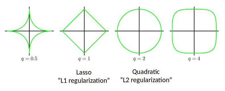
L2 regularization is also called Ridge Regression.
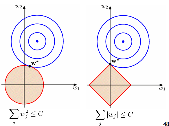
Regularized Least Squares: Comparison
- At the solution the contours are always tangent to each other.
- Lasso tends to generate sparser solutions than a quadratic regularizer.
Another explanation for L2 regularization, using Fourier analysis: https://arxiv.org/abs/1806.08734v1
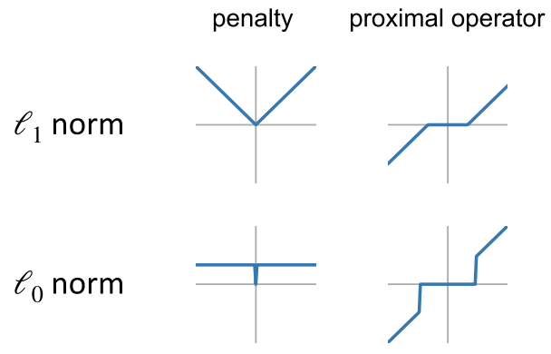
Extra: Solving the L1 case
- The L2 regularization $\|w\|_2^2$ is smooth and differentiable, and hence easy to solve.
- But how about the L1 case $\|w\|_1$? The objective is not differentiable whenever one $w_j$ is zero.
Here we briefly discuss the Proximal Gradient Descent (PGD) method to solve this problem.
The algorithm
Formally, let's consider $$ \min_w F(w) = h(w) + r(w) $$ where $h(w)$ is differentiable and $r(w)$ is not. In the L1 example,
$$ h(w) = \|\Phi w-t\|^2,\quad r(w) = \lambda \|w\|_1 $$
But here we still assume both $h$ and $r$ are convex.
In short, PGD does the following, $$ w_{k+1} = \text{prox}_{\alpha r}(w_k - \alpha\nabla h(w_k)) $$
- Regular GD for $h$ with a step size $\alpha$
- A special "proximal operator" for $r$
The proximal operator does the following, $$ \text{prox}_{\alpha r}(v) = \arg\min_{u} \frac{1}{2}\|u-v\|^2 + \alpha r(u) $$
- $v$ is the update based on the smooth part of objective
- $u$ is the modification to $v$ considering the non-smooth part
- $u$ is as close to $v$ as possible (1st term), while minimizing $r$ (2nd term)
For typical regularizers, the proximal operators have closed-form solutions.
For example, in the L0 case, we simply zero out values smaller than a threshold.
How it works
Recall, if the objective were differentiable, e.g., without $r(w)$, the optimality condition is simply $$ \nabla F(w) = \nabla h(w) = 0 $$
From the optimality condition, if we have an iterate $w_k$, the next iterate that we pick satisfies $$ 0 = \nabla h(w_{k+1}) \approx \nabla h(w_k) + \frac{w_{k+1} - w_k}{\alpha} \quad\Rightarrow \quad w_{k+1} = w_k - \alpha \nabla h(w_k) $$
In the non-differentiable case, the optimality condition generalizes to $$ \partial F(w) = \nabla h(w) + \partial r(w)\quad\text{and}\quad 0\in \partial F(w) $$ where $\partial r(w)$ is a special notation called subgradient - a set of vectors $g$ such that for all $v$ $$ r(v) \geq r(w) + g^T (v-w) $$
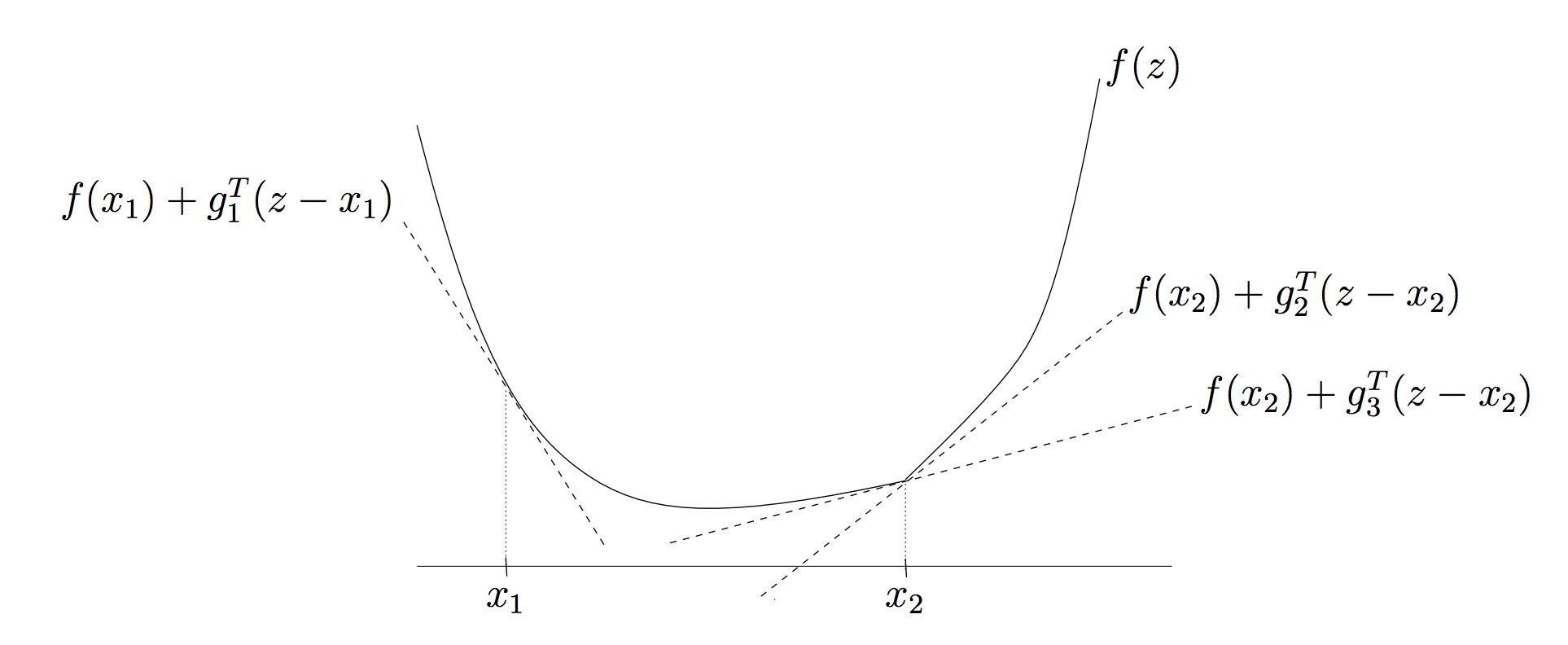
In analogy to the smooth case, during iterations, we would like $$ 0\in \partial F(w) = \nabla h(w_{k+1}) + \partial r(w_{k+1}) \approx \nabla h(w_k) + \frac{w_{k+1} - w_k}{\alpha} + \partial r(w_{k+1}) $$
If we choose $$ v = w_k - \alpha\nabla h(w_k),\quad u = w_{k+1} $$ then optimality condition is equivalent to $$ 0\in (u-v) + \alpha\partial r(u) $$
But the above is exactly the subgradient in the proximal step: $$ (u-v) + \alpha \partial r(u) = \partial\left( \frac{1}{2}\|u-v\|^2 + \alpha r(u) \right) $$
In other words, the following two are equivalent:
- Evaluating the proximal step
- Satisfying the optimality condition of the original problem (up to the first-order approximation)
Scalar example
Next we take a scalar L1 case as an example, so $\|w\|_1=|w|$, and let $w^*$ be a constant, $$ \min_w \frac{1}{2}(w-w^*)^2 + \lambda |w| $$
If $\lambda=0$, the solution is apparently $w=w^*$.
We want $$ 0\in w-w^* + \lambda \partial |w| $$
If $w>0$, then $\partial |w|=\nabla w=1$, and the equation simplifies $$ 0 = w-w^* + \lambda \Rightarrow w = w^* - \lambda $$
But this relation requires $w>0$, or $w^* > \lambda$.
So, when $w^* > \lambda$, the solution is $w = w^* - \lambda$.
If $w<0$, similarly, we would get: when $w^* < -\lambda$, the solution is $w = w^* + \lambda$.
If $w=0$, then $\partial |w|=[-1,1]$, and $$ 0\in w-w^* + \lambda [-1, 1] = -w^* + [-\lambda, \lambda]\quad \text{or}\quad w^* \in [-\lambda, \lambda] $$ This means, when $|w^*|\leq \lambda$, we simply zero out $w=0$ - this is where the sparsity comes in.
The above recovers the L1 proximal operator.
Some notes
- More information on proximal gradient method wiki and an introductory text
Examples: Regularized regression
Ridge Regression
rdg_sc, rdg_coef = fitModel(1.0, lm.Ridge)

Lasso
las_sc, las_coef = fitModel(0.01, lm.Lasso)

LR vs Ridge vs Lasso
ii = np.arange(13)
f = plt.figure(figsize=(6,4))
plt.semilogy(ii, np.abs(_cs[11]), 'r--', label='LR')
plt.semilogy(ii, np.abs(rdg_coef), 'b-', label='Ridge')
plt.semilogy(ii, np.abs(las_coef), 'g-', label='Lasso')
plt.legend()
_=plt.xlabel(r'$w_i$')

Bad choice of hyperparameter
_, _ = fitModel(1e-8, lm.Ridge)

_, _ = fitModel(1e8, lm.Ridge)

Choosing the best hyperparameter
f = plt.figure()
plt.plot(np.log(lams), errs[0], 'b-', label='Training error')
plt.plot(np.log(lams), errs[1], 'r-', label='Test error')
plt.xlabel(r'$\log(\lambda)$')
_=plt.ylabel('1-R2')

Ridge Regularization: $E_{RMS}$ vs $\ln\lambda$
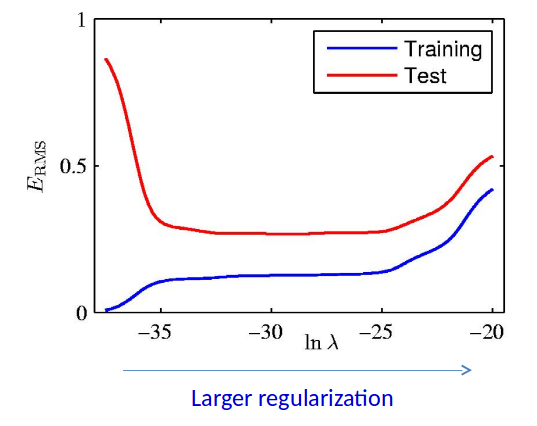
NOTE: For simplicity of presentation, we divided the data into training set and test set. However, it’s not legitimate to find the optimal hyperparameter based on the test set. We will talk about legitimate ways of doing this when we cover model selection and cross-validation.
Regularized Least Squares: Summary
- Simple modification of linear regression
- L2 Regularization controls the tradeoff between fitting error and complexity.
- Small L2 regularization results in complex models, but with risk of overfitting
- Large L2 regularization results in simple models, but with risk of underfitting
- It is important to find an optimal regularization that balances between the two
- More on model selection in future lectures
One more model... Elastic net
- Combination of Ridge and Lasso $$ \widetilde{E}(w) = \frac12 \sum_{n=1}^N (w^T \phi(x^{(n)}) - t^{(n)})^2 + \lambda\left( \frac{1-\alpha}{2} \sum_{j=1}^M |w_j|^2 + \alpha\sum_{j=1}^M |w_j| \right) $$
- Works better when the features are correlated.
- More details:
- [MLaPP] Chp. 13.5.3
- H. Zou and T. Hastie, Regularization and variable selection via the elastic net, 2005
Yet more models...
The bias of the Lasso estimate for a truly nonzero variable is about $\lambda$ for large regression coefficients coefficients.
To fix the issue: Adaptive Lasso, MCP, SCAD
- for those who are interested: https://myweb.uiowa.edu/pbreheny/7600/s16/notes/2-29.pdf
When it comes to deep learning
We will see Double-Descent phenomenon - Errors in training and test both decrease as number of features increase.
To be discussed more later in this module.