Math_LA slides

Machine Learning for Engineering¶

Math Background: Linear Algebra¶

Instructor: Daning Huang¶

TODAY: Quick (re)view of linear algebra¶

Vectors and Matrices
Eigenvalue decomposition
Singular value decomposition (SVD)

References:¶

[Kreyszig] Chap. 7-8
[PRML] Appendix C
Matrix Norms

Vector norms¶

Perhaps the most common norm is the Euclidean norm $$ \|x\|_2 := \sqrt{x_1^2 + x_2^2 + \ldots x_n^2}$$

This is a special case of the $p$-norm: $$ \|x\|_p := \left(|x_1|^p + \ldots + |x_n|^p\right)^{1/p}$$

Special cases: $p=1$ and $p=0$? $$ \|x\|_1\ \mbox{Sum of absolute values},\quad \|x\|_0\ \mbox{Number of non-zeros} $$

There's also the so-called infinity norm $$ \|x\|_\infty := \max_{i=1,\ldots, n} |x_i|$$

A vector $x$ is said to be normalized if $\|x\| = 1$

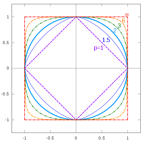
Geometrical interpretation¶

In 2D, when $\|x\|=1$, what is the shape of curve?

Matrix norms¶

Simple extension from vector norms - think a $m\times n$ matrix as a $mn$-dimensional vector
- For example, Frobenius norm $$ \|A\|_F := \left( \sum_{i,j} A_{ij}^2 \right)^{1/2} $$

Induced norms from vector norms $$ \|A\|_p := \max_{\|x\|_p=1}\|Ax\|_p $$

Orthogonal + Normalized = Orthonormal¶

Two vectors $x,y$ are orthogonal if $x^T y = 0$
A square matrix $U \in \mathbb{R}^{n \times n}$ is orthogonal if all columns $u_1, \ldots, u_n$ are orthogonal to each other (i.e. $u_i^\top u_j = 0$ for $i \ne j$)
$U$ is orthonormal if it is orthogonal and the columns are normalized, i.e. $\|u_i\|_2 = 1$ for every $i$.
$U$ forms an orthonormal basis of the $\mathbb{R}^n$ vector space.

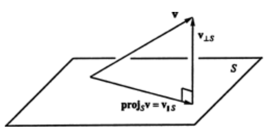
Orthonormal matrix for projection¶

$U\in \mathbb{R}^{n\times m}$ column-wise orthonormal, i.e. $U^\top U=I_m$
Then $U$ form the orthonormal basis of a $m$-dimensional subspace $S$ in $\mathbb{R}^n$
- e.g. 2D plane in 3D space
The component $p$ of a $n$-dimensional vector $v$ in subspace $S$ is given by the projection $ p=UU^\top v $
The residual is $r = v-p = (I-UU^\top)v$ and orthogonal to $p$
- Or - the residual does not carry any information concerning the subspace

Positive Definiteness¶

We say a symmetric matrix $A$ is positive definite if $$ x^\top A x > 0 \text{ for all } x \ne 0$$
We say a matrix is positive semi-definite (PSD) if $$ x^\top A x \geq 0 \text{ for all } x$$
A matrix that is positive definite gives us a norm. Let $$ \| x \|_A := \sqrt{x ^\top A x} $$

Visualization of PD matrices¶

Contour plots of $f(x)=x^TAx$, starting with -

$$ A=\begin{bmatrix} 1 & 0 \\ 0 & 4 \end{bmatrix} $$

In [3]:

A = np.array([
    [1,1],
    [1,4]])
pltPSD(A, with_eig=False, if3d=False)
pltPSD(A, with_eig=False, if3d=True)

Eigenvalues and Eigenvectors¶

What are eigenvectors?¶

A Matrix is a mathematical object that acts on a (column) vector, resulting in a new vector, i.e. $Ax=b$
An eigenvector is the resulting vector that is parallel to $x$ (some multiple of $x$) $$ {A}x=\lambda x $$
The eigenvectors with an eigenvalue of zero are the vectors in the nullspace
If A is singular (takes some non-zero vector into 0) then $\lambda=0$

Numerical example¶

In [4]:

X = np.array([[3, 1], [1, 3]])
Matrix(X)

Out[4]:

$\displaystyle \left[\begin{matrix}3 & 1\\1 & 3\end{matrix}\right]$

In [5]:

eigenvals, eigenvecs = np.linalg.eig(X)
Matrix(eigenvecs)

Out[5]:

$\displaystyle \left[\begin{matrix}0.707106781186547 & -0.707106781186547\\0.707106781186547 & 0.707106781186547\end{matrix}\right]$

In [6]:

newX = eigenvecs.dot(np.diag(eigenvals)).dot(eigenvecs.T)
Matrix(newX)

Out[6]:

$\displaystyle \left[\begin{matrix}3.0 & 1.0\\1.0 & 3.0\end{matrix}\right]$

Let $A$ be a matrix whose eigenvalues are $\lambda_1, \ldots, \lambda_n$
Then we have the trace of satisfying $$\text{tr}(A) = \sum_{i=1}^n \lambda_i$$

In [7]:

X = np.random.randn(5,10)
A = X.dot(X.T) # For fun, let's look at A = X * X^T
eigenvals, eigvecs = np.linalg.eig(A) # Compute eigenvalues of A
sum_of_eigs = sum(eigenvals) # Sum the eigenvalues
trace_of_A = A.trace() # Look at the trace
(sum_of_eigs, trace_of_A) # Are they the same?

Out[7]:

$\displaystyle \left( 38.2082852673183, \ 38.2082852673183\right)$

Let $A$ be a matrix whose eigenvalues are $\lambda_1, \ldots, \lambda_n$
Then we have the trace of satisfying $$|A| = \prod_{i=1}^n \lambda_i$$

In [8]:

# We'll use the same matrix A as before
prod_of_eigs = np.prod(eigenvals) # Sum the eigenvalues
determinant = np.linalg.det(A) # Look at the trace
(prod_of_eigs, determinant) # Are they the same?

Out[8]:

$\displaystyle \left( 4630.30937169143, \ 4630.30937169142\right)$

Eigenvalue Decomposition¶

Let $A$ be a matrix whose eigenvalues are $\lambda_1, \ldots, \lambda_n$ $$\Lambda=Diag([\lambda_1, \ldots, \lambda_n])$$
And the corresponding eigenvectors are $x_1, \ldots, x_n$ $$X=[x_1, \ldots, x_n]$$
Then we have the following decomposition $$ A=X\Lambda X^{-1} $$
Further if $X$ is orthonormal, i.e. $X^{-1}=X^\top$, $$ A=\sum_{i=1}^n \lambda_i x_i x_i^\top $$

Round back to visualization

In [9]:

A = np.array([
    [1,1],
    [1,2]])
pltPSD(A, with_eig=True, if3d=False)

Singular Value Decomposition¶

Not all square matrices can do eigenvalue decomposition - but
Any matrix (symmetric, non-symmetric, etc.) $A \in \mathbb{R}^{n\times m}$ admits a singular value decomposition (SVD)
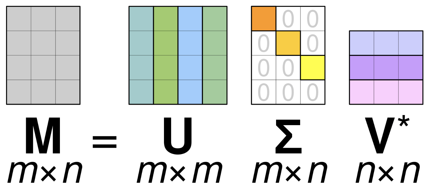
The decomposition has three factors, $U \in \mathbb{C}^{n \times n}$, $\Sigma \in \mathbb{R}^{n \times m}$, and $V \in \mathbb{C}^{m \times m}$ $$A = U \Sigma V^*$$
$U$ and $V$ are both orthonormal matrices, and $\Sigma$ is diagonal. $V^*$ indicates conjugate transpose.

SVD Example¶

In [10]:

A = np.array([[4, 4], [-3, 3]])
Matrix(A)

Out[10]:

$\displaystyle \left[\begin{matrix}4 & 4\\-3 & 3\end{matrix}\right]$

Let's show Sigma from the SVD output

In [11]:

U, Sigma_diags, V = np.linalg.svd(A)
Matrix(np.diag(Sigma_diags)) # Numpy's SVD only returns diagonals, here I'm showing full Sigma

Out[11]:

$\displaystyle \left[\begin{matrix}5.65685424949238 & 0\\0 & 4.24264068711928\end{matrix}\right]$

And we can show the orthonormal bases $U$ and $V$

In [13]:

Matrix(U), Matrix(V) # I rounded the values for clarity

Out[13]:

$\displaystyle \left( \left[\begin{matrix}-1.0 & 0\\0 & 1.0\end{matrix}\right], \ \left[\begin{matrix}-0.70711 & -0.70711\\-0.70711 & 0.70711\end{matrix}\right]\right)$

Properties of the SVD¶

For simplicity, let's assume everything is real; then conjugate transpose is just transpose.

$$\text{SVD:} \quad \quad A = U \Sigma V^\top$$

The singular values of $A$ are the diagonal elements of $\Sigma$
The singular values of $A$ are the square roots of the eigenvalues of both $A^\top A$ and $A A^\top$
The left-singular vectors of $A$, i.e. the columns of $U$, are the eigenvectors of $A A^\top$
The right-singular vectors of $A$, i.e. the columns of $V$, are the eigenvectors of $A^\top A$

Also - $\|A\|_2 = \sigma_\max(A)$, $\|A\|_F = (\sum_{i=1}^n \sigma_i^2)^{1/2}$

An analogy to eigenvalue decomposition - but applicable to all matrices $$ A=\sum_{i=1}^{n} \sigma_iu_iv_i^\top $$

Common trick to truncate and approximate a matrix - say the last $m$ $\sigma$'s are close to zero

$$ A\approx\sum_{i=1}^{n-m} \sigma_iu_iv_i^\top := \hat{A} $$

Error estimate

$$ \frac{\|A-\hat{A}\|_F^2}{\|A\|_F^2} = \frac{\sum_{i=n-m+1}^{n}\sigma_i^2}{\sum_{i=1}^{n}\sigma_i^2} $$

What is the implication in (1) subspace projection and (2) data compression?

Simple application of SVD: Condition number¶

Consider two sets of linear equations $$ \begin{bmatrix} 3 & 1 \\ -3.0001 & 1 \end{bmatrix} \begin{bmatrix} x_1 \\ x_2 \end{bmatrix} = \begin{bmatrix} 4 \\ 4.0001 \end{bmatrix} $$

$$ \begin{bmatrix} 3 & 1 \\ -2.9999 & 1 \end{bmatrix} \begin{bmatrix} x_1 \\ x_2 \end{bmatrix} = \begin{bmatrix} 4 \\ 4.0002 \end{bmatrix} $$

How different are their solutions?

In [14]:

A1=np.array([
    [3,1],
    [-3.0001,1]])
b1=np.array([4,4.0001])

A2=np.array([
    [3,1],
    [-2.9999,1]])
b2=np.array([4,4.0002])

x1=np.linalg.solve(A1,b1)
x2=np.linalg.solve(A2,b2)

print(x1)
print(x2)

[-1.66663889e-05  4.00005000e+00]
[-3.33338889e-05  4.00010000e+00]

Consider another two sets of linear equations - note the signs $$ \begin{bmatrix} 3 & 1 \\ 3.0001 & 1 \end{bmatrix} \begin{bmatrix} x_1 \\ x_2 \end{bmatrix} = \begin{bmatrix} 4 \\ 4.0001 \end{bmatrix} $$

$$ \begin{bmatrix} 3 & 1 \\ 2.9999 & 1 \end{bmatrix} \begin{bmatrix} x_1 \\ x_2 \end{bmatrix} = \begin{bmatrix} 4 \\ 4.0002 \end{bmatrix} $$