Machine Learning for Engineering

Math Background: Optimization

Instructor: Daning Huang

TODAY: Quick (re)view of optimization

• Convexity
• KKT condition
• Dual problems

References:

• [Kreyszig] Chap. 22-23
• [PRML] Appendix E
• More details: Convex Optimization, Boyd and Vandenberghe

Functions and Convexity

• Let $f$ be a function mapping $\mathbb{R}^{n} \to \mathbb{R}$, and assume $f$ is twice differentiable.
• The gradient and hessian of $f$, denoted $\nabla f(x)$ and $\nabla^2 f(x)$, are the vector and matrix functions: $$\nabla f(x) = \begin{bmatrix}\frac{\partial f}{\partial x_1} \\ \vdots \\ \frac{\partial f}{\partial x_n}\end{bmatrix} \quad \quad \quad \nabla^2 f(x) = \begin{bmatrix}\frac{\partial^2 f}{\partial x_1^2} & \ldots & \frac{\partial^2 f}{\partial x_1 \partial x_n} \\ \vdots & & \vdots \\\frac{\partial^2 f}{\partial x_1 \partial x_n} & \ldots & \frac{\partial^2 f}{\partial x_n^2}\end{bmatrix}$$
• Note: the hessian is always symmetric!

Gradients of three simple functions

• Let $b$ be some vector, and $A$ be some symmetric matrix
• $f(x) = b^{\top} x \implies \nabla_x f(x) = b$
• $f(x) = x^{\top} A x \implies \nabla_x f(x) = 2 A x$
• $f(x) = x^{\top} A x \implies \nabla^2_x f(x) = 2A$

Convex functions

• We say that a function $f$ is convex if, for any distinct pair of points $x,y$ we have $$f\left(\frac{x + y}{2}\right) \leq \frac{f(x)}{2} + \frac{f(y)}{2}$$

• Illustration

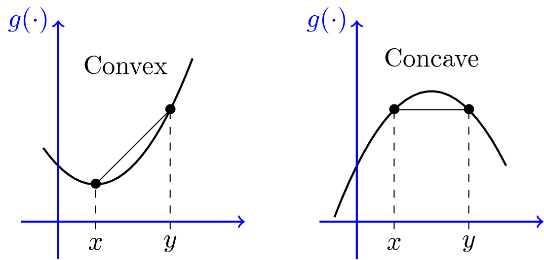
Properties of convex functions

• If $f$ is differentiable, then $f$ is convex iff $f$ "lies above its linear approximation", i.e.: $$ f(x + y) \geq f(x) + \nabla_x f(x) \cdot y \quad \text{ for every } x,y$$
• If $f$ is twice-differentiable, then the hessian is always positive semi-definite (PSD)!
• Show this last one as an exercise :-)

Convex Sets

• $C \subseteq \mathbb{R}^n$ is convex if $$t x + (1-t)y \in C$$ for any $x, y \in C$ and $0 \leq t \leq 1$
• that is, a set is convex if the line connecting any two points in the set is entirely inside the set

A Generic Optimization Problem

Assume $f$ is some function, and $C \subset \mathbb{R}^n$ is some set. The following is an optimization problem: $$ \begin{array}{ll} \mbox{minimize} & f(x) \\ \mbox{subject to} & x \in C \end{array} $$

• How hard is it to find a solution that is (near-) optimal? This is one of the fundamental problems in many engineering applications.
• A huge portion of machine learning relies on this task

A rough optimization hierarchy

$$ \mbox{minimize } f(x) \quad \mbox{subject to } x \in C $$

• [Really Easy] $C = \mathbb{R}^n$ (i.e. problem is unconstrained), $f$ is differentiable and strictly convex
• [Easyish] $C = \mathbb{R}^n$, $f$ is convex
• [Medium] $C$ is a convex set, $f$ is convex
• [Hard] $C$ is a convex set, $f$ is non-convex
• [REALLY Hard] $C$ is an arbitrary set, $f$ is non-convex

Optimization without constraints

$$ \begin{array}{ll} \mbox{minimize} & f(x) \\ \mbox{subject to} & x \in \mathbb{R}^n \end{array} $$

• This problem tends to be easier than constrained optimization
• We just need to find an $x$ such that $$\nabla f(x) = 0$$
• Gradient-based algorithms: gradient descent or Newton's method. (More on this in Neural Networks)

Example

$$ \begin{array}{ll} \mbox{minimize} & f(x)=x_1^2+x_2^2+1 \\ \mbox{subject to} & x \in \mathbb{R}^2 \end{array} $$

• Minimizer: Let $\nabla f(x)=0$, $x^*=[0,0]$.

x = np.linspace(-1,1,51)
X, Y = np.meshgrid(x, x)
F = X**2+Y**2+1
f = plt.figure()
c = plt.contour(X, Y, F, 10)
plt.colorbar(c)
plt.plot(0,0,'bo')
_=plt.text(0.1,0,'x*',fontsize=12)

Optimization with constraints

$$ \begin{array}{ll} \mbox{minimize} & f(x) \\ \mbox{subject to} & g_i(x) \leq 0, \quad i = 1, \ldots, m \end{array} $$

Here the set $C := \{ x : g_i(x) \leq 0, i=1, \ldots, m \}$

Two cases:

• The solution of this optimization may occur in the interior of $C$, in which case the optimal $x$ will have $\nabla f(x) = 0$
• But what if the solution occurs on the boundary of $C$?

Solution on the boundary - Equality constraints

• Without loss of generality, consider one constraint: $$ \begin{array}{ll} \mbox{minimize} & f(x) \\ \mbox{subject to} & g(x) = 0 \end{array} $$

• Note that at minimizer $$ \nabla f \parallel \nabla g,\quad \rightarrow\quad \nabla f + \lambda\nabla g = 0,\quad \lambda\neq 0 $$

• Convert to an unconstrained problem using Lagrangian $$ \begin{array}{ll} \mbox{minimize} & L(x,\lambda) = f(x) + \lambda g(x) \end{array} $$

• The solution is found by $$ \begin{array}{ll} \nabla_x L(x,\lambda) &= 0 \\ \nabla_\lambda L(x,\lambda) &= 0 \end{array} $$

Example

$$ \begin{array}{ll} \mbox{minimize} & f(x)=x_1^2+x_2^2+1 \\ \mbox{subject to} & -1/2+x_1+x_2=0 \end{array} $$

Lagrangian: $L(x,\lambda)=(x_1^2+x_2^2+1)+\lambda(-1/2+x_1+x_2)$

Minimizer: $x^*=[1/4,1/4]$.

g = 0.5-x
f = plt.figure()
c = plt.contour(X, Y, F, 10)
plt.colorbar(c)
plt.plot(x, g, 'r--')
plt.plot(0.25,0.25,'bo')
plt.text(0.15,0.15,'x*',fontsize=12)
_=plt.ylim([-1,1])

Adding inequality constraints

• Without loss of generality, consider one constraint: $$ \begin{array}{ll} \mbox{minimize} & f(x) \\ \mbox{subject to} & g(x) \leq 0 \end{array} $$

• Inactive constraint: If the minimizer is inside the boundary, i.e. $g(x)>0$, then it is effectively unconstrained. Like before, $$ \nabla f = 0,\quad \mbox{i.e. } \lambda=0 $$

• Active constraint: If the minimizer is on the boundary, i.e. $g(x)=0$, then we can solved it (again) by: $$ \nabla f + \lambda\nabla g = 0,\quad \lambda>0 $$

• Above discussion summarizes the necessary conditions for optimality, i.e. the Karush-Kuhn-Tucker (KKT) conditions (for the one-inequality-constraint case) $$ \begin{array}{rl} \nabla_x L(x,\lambda) &= 0 \\ g(x) &\leq 0 \\ \lambda &\geq 0 \\ \lambda g(x) &= 0 \end{array} $$

Example

$$ \begin{array}{ll} \mbox{minimize} & f(x)=x_1^2+x_2^2+1 \\ \mbox{subject to} & -1/2+x_1+x_2 \leq 0 \end{array} $$

Lagrangian: $L(x,\lambda)=(x_1^2+x_2^2+1)+\lambda(-1/2+x_1+x_2)$

Minimizer: $x^*=[0,0]$.

h = -1*np.ones_like(x)
f = plt.figure()
c = plt.contour(X, Y, F, 10)
plt.colorbar(c)
plt.fill_between(x, h, g, color='g', alpha=0.3)
plt.plot(0.0,0.0,'bo')
plt.text(0.1,0.0,'x*',fontsize=12)
_=plt.ylim([-1,1])

Python example

Using vanilla SciPy optimizer

# Function to be minimized
def fun(x):
    return x[0]**2 + x[1]**2 + 1

# Constraint function
# BE CAREFUL: For inequalities, non-negative values are assumed
def cnst(x):
    return 0.5 - x[0] - x[1]

# Initial guess
x0 = [2.0, 2.0]

# Unconstrained problem
# Note the number of evaluations of the function and its jacobian
sol0 = minimize(fun, x0)
print(sol0)

      fun: 1.000000000000016
 hess_inv: array([[ 0.75000001, -0.24999999],
       [-0.24999999,  0.75000001]])
      jac: array([-1.63912773e-07, -1.63912773e-07])
  message: 'Optimization terminated successfully.'
     nfev: 9
      nit: 2
     njev: 3
   status: 0
  success: True
        x: array([-8.93115557e-08, -8.93115557e-08])

# Equality constrained problem
c1 = {'type': 'eq', 'fun': cnst}
sol1 = minimize(fun, x0, constraints=(c1,))
print(sol1)

     fun: 1.125
     jac: array([0.5, 0.5])
 message: 'Optimization terminated successfully'
    nfev: 6
     nit: 2
    njev: 2
  status: 0
 success: True
       x: array([0.25, 0.25])

# Inequality constrained problem
c2 = {'type': 'ineq', 'fun': cnst}
sol2 = minimize(fun, x0, constraints=(c2,))
print(sol2)

     fun: 1.0
     jac: array([1.49011612e-08, 1.49011612e-08])
 message: 'Optimization terminated successfully'
    nfev: 7
     nit: 2
    njev: 2
  status: 0
 success: True
       x: array([0., 0.])

General Treatment: Lagrange Duality

. $$ \begin{array}{ll} \mbox{minimize} & f(x) \\ \mbox{subject to} & g_i(x) \leq 0, \quad i = 1, \ldots, m \end{array} $$

• Working with the Lagrangian: $$ L(x,\boldsymbol{\lambda}) := f(x) + \sum_{i=1}^m \lambda_i g_i(x) $$
• The vector $\boldsymbol{\lambda} \in \mathbb{R}^{m+}$ are dual variables
• For fixed $\boldsymbol{\lambda}$, we now solve $\nabla_x L(x,\boldsymbol{\lambda}) = \mathbf{0}$

• Assume, for every fixed $\lambda$, we found $x_\lambda$ such that $$ \nabla_x L(x_\lambda,\boldsymbol{\lambda}) = \nabla f(x_\lambda) + \sum_{i=1}^m \lambda_i \nabla g_i(x_\lambda) = \mathbf{0}$$
• Now we have what is called the dual function, $$h(\boldsymbol{\lambda}) = \inf_x L(x,\lambda) = L(x_\lambda,\boldsymbol{\lambda})$$

The Lagrange Dual Problem

• What did we do here? We took one optimization problem: $$ p^* := \begin{array}{ll} \mbox{minimize} & f(x) \\ \mbox{subject to} & g_i(x) \leq 0, \quad i = 1, \ldots, m \end{array} $$

• And then we got another optimization problem: $$ d^* := \begin{array}{ll} \mbox{maximize} & h(\boldsymbol \lambda) \\ \mbox{subject to} & \lambda_i \geq 0, \quad i = 1, \ldots, m \end{array} $$

• Sometimes this dual problem is easier to solve, since it is always convex
• We always have weak duality: $p^* \geq d^*$
• Under nice conditions, we get strong duality: $p^* = d^*$