Definition of Probability¶
- [Sample Space], $\Omega$, $S$
- Set, Possible outcomes
- [Event Space], $\mathcal{F}$, $E$
- Collection of subsets, Things having probabilities
- [Probability Measure], $P$, $\pi$
- Area/Measure, Map things to probability
- [Probability Space], $(\Omega,\mathcal{F},P)$
- A triple
Example 0¶
Roll a dice of 10 faces - What are $\Omega$, $\mathcal{F}$, and $P$?
Properties of probability¶
Axioms
- $P(A)\geq 0,\quad \forall A\in \mathcal{F}$
- $P(\Omega)=1$
- If $A_1,A_2,\cdots$ are disjoint events, then $P(\cup_i A_i)=\sum_i P(A_i)$
Other properties:
If $A\subset B$, $P(A)\leq P(B)$
$P(A\cap B)\leq \min(P(A),P(B))$
Union bound: $P(A\cup B)\leq P(A)+P(B)$
Complement set: $P(\Omega\backslash A)=1-P(A)$
Conditional Probability¶
- Chain rule: $P(A\cap B)=P(A|B)P(B)$
- For events $A,B\in\mathcal{F}$ with $P(B)>0$, conditional probability of $A$ given $B$ is $$ P(A|B)=\frac{P(A\cap B)}{P(B)} $$
- The outcome is definitely in $B$, so $B$ becomes the new sample space.
Independence¶
Independence $A\perp B$:
- Events $A$ and $B$ are independent if $P(A\cap B)=P(A)P(B)$.
- If $P(A)>0$, then it means $P(B|A)=P(B)$
Conditional independence $A\perp B|C$:
- Events $A$ and $B$ are conditionally independent given $C$ if $$ P(A\cap B|C)=P(A|C)P(B|C) $$
- If $P(A)>0$, then it means $P(B|A,C)=P(B,C)$.
Example 1¶
Roll a dice of 10 faces
- Let $A=\{1,2,\cdots,5\}$, $B=\{\mbox{even number}\}$, $C=\{5,6,\cdots,10\}$
- What is $P(A\cap B)$?
- What is $P(A|C)$?
- Is $A\perp B$?
- Give an example of $D$ such that $A\perp B|D$.
Bayes' Rule¶
- From chain rule: $P(A\cap B)=P(A|B)P(B)=P(B|A)P(A)$ $\rightarrow$ $$ P(B|A)=\frac{P(A|B)P(B)}{P(A)} $$
- More general form: $$ P(B_i|A)=\frac{P(A|B_i)P(B_i)}{\sum_i P(A|B_i)P(B_i)} $$ where $\cup_i B_i=\Omega$
- In statistics, $B_i$ is "hypothesis" and $A$ is "evidence"
- In machine learning, $B_i$ is "model" and $A$ is "data"
- Prior $P(B_i)$: How probable is the model before observation
- likelihood $P(A|B_i)$: How probable is the data given a model
- Marginal $P(A)$: How probable is the data given all possible models
- Posterior $P(B_i|A)$: How probable is the model given the data - and we pick the most likely one
Example 2¶
(Statistics flavor)
Consider a dice of 4 faces, and you were told the numbers are either all even or all odd.
- Hypothesis: $B_1=\{2,4,6,8\}$ and $B_2=\{1,3,5,7\}$; no special prior - half and half
- Evidence: $A=\{1,2,4,6\}$
- Given the evidence how likely are the numbers all even?
Random Variables¶
- Essentially, RV is a function $X:\Omega\rightarrow \mathbb{R}^d$
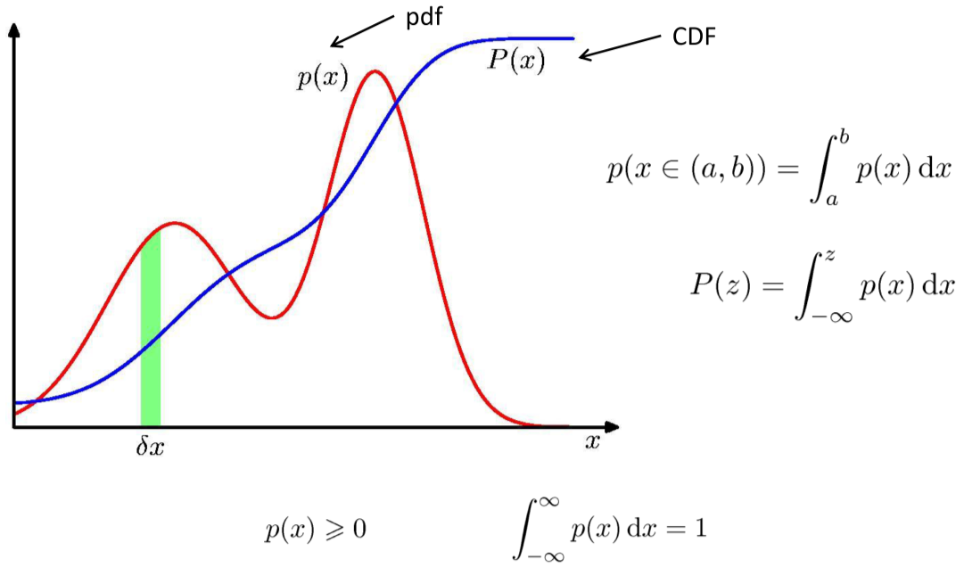
- Can be characterized by Cumulative Distribution Function (CDF), $X\sim F_X$ $$ F_X(x) = P(X\leq x) $$
- Identical distribution: RVs having the same CDF.
Probability distribution function (PDF)¶
- When CDF is continuous, one can define PDF as $$ f_X(x) = \frac{d}{dx}F_X(x) $$
- Then $$ P(a<X<b)=\int_a^b f_X(x)dx $$
- Be careful, for continuous RV, $P(X=c)=0$
Expectation¶
For continuous RV,
- "Average outcome", or mean: $\mu=\mathbb{E}[x]=\int p(x)xdx$
- General form: $$ \mathbb{E}[f]=\int p(x)f(x)dx $$
- Conditional expectation: $$ \mathbb{E}_x[f|y]=\int p(x|y)f(x)dx $$
Properties:
- $\mathbb{E}[af(X)]=a\mathbb{E}[f(X)]$
- $\mathbb{E}[f(X)+g(X)]=\mathbb{E}[f(X)]+\mathbb{E}[g(X)]$
Variance¶
"Spread-out in outcome": $\sigma^2=Var[X]=\mathbb{E}[X-\mathbb{E}[X]]^2$
Alternative form: $\mathbb{E}[X-\mathbb{E}[X]]^2 = \mathbb{E}[X^2]-\mathbb{E}[X]^2$
$Var[af(X)]=a^2Var[f(X)]$
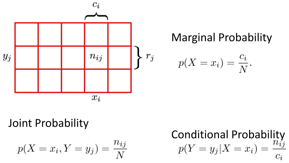
Multiple Random Variables¶
- Joint PDF: $f_{X,Y}(x,y)$, so that $$ P(x_1<X<x_2, y_1<Y<y_2)=\int_{x_1}^{x_2}\int_{y_1}^{y_2}f_{X,Y}(x,y)dxdy $$
- Marginalizing - Extracting a single RV: $$ f_X(x)=\int_{\mathcal{Y}}f_{X,Y}(x,y)dy $$
- Conditioning $$ f_{X|Y}(x|y) = \frac{f_{X,Y}(x,y)}{f_Y(y)} = \frac{f_{X,Y}(x,y)}{\int_{\mathcal{X}} f_{X,Y}(x,y)dx} $$
Expectation and covariance¶
For two continuous RV's,
- Expectation: $$ \mathbb{E}[g(X,Y)]=\int_{\mathcal{X}}\int_{\mathcal{Y}} f_{X,Y}(x,y)g(x,y)dxdy $$
- Covariance - correlation between RV's, $$ Cov[X,Y] = \mathbb{E}[(X-\mathbb{E}[X])(Y-\mathbb{E}[Y])] $$ Alternatively, $$ Cov[X,Y]=\mathbb{E}[XY]-\mathbb{E}[X]\mathbb{E}[Y] $$
More properties:
$Var[X+Y]=Var[X]+Var[Y]+2Cov[X,Y]$
If $X$ and $Y$ are independent, $Cov[X,Y]=0$
and $\mathbb{E}[f(X)g(Y)]=\mathbb{E}[f(X)]\mathbb{E}[g(Y)]$
Likelihood - Bayes rule again¶
- Likelihood function, $p(D|w)$, is evaluated for observed data $D$ as a function of $w$. "How possible is the observation given the parameter"
- Bayes' rule: $p(w|D)\propto p(D|w) \times p(w)$
- In words: Posterior $\propto$ Likelihood $\times$ Prior
Maximum Likelihood
- Find $w^*$ to maximize the likelihood function $p(D|w)$.
- This maximizes the probability of the observed data.
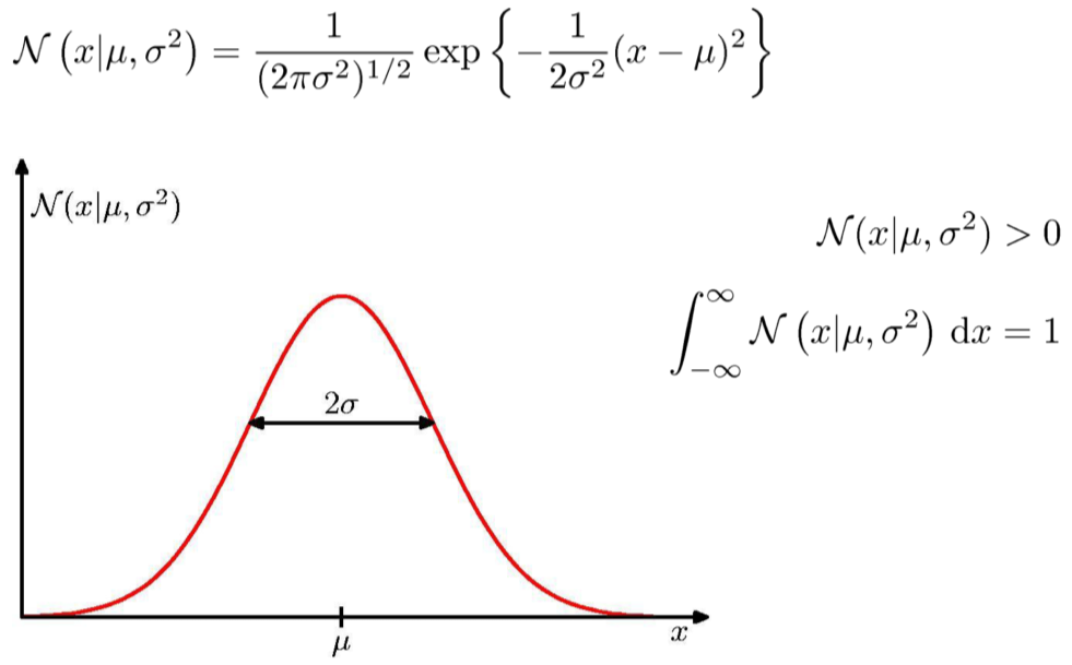
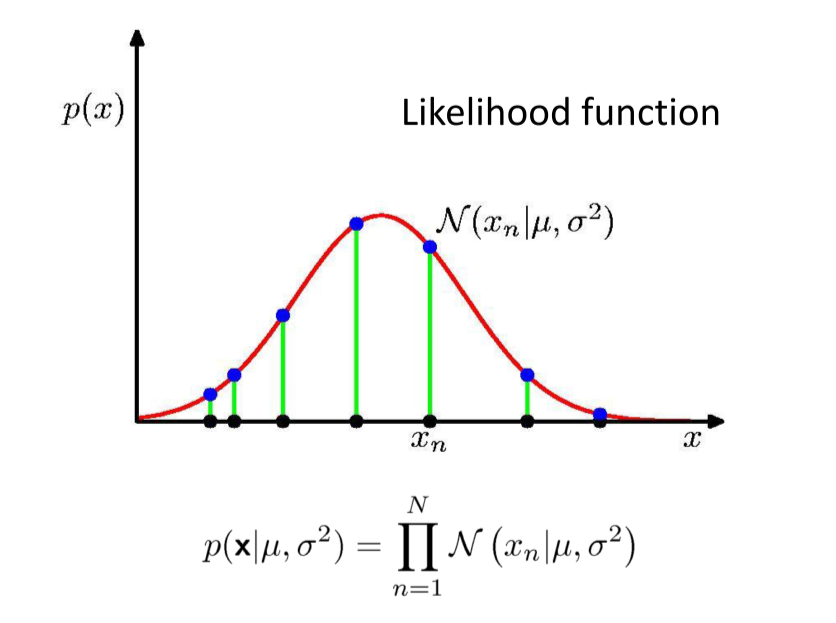
Example: Gaussian distribution¶
- Data $D=\{x_1,\cdots,x_N\}$
- Drawn from Gaussian distribution $$ \mathcal{N}(x|\mu,\sigma^2)=\frac{1}{\sqrt{2\pi}\sigma}\exp\left\{-\frac{(x-\mu)^2}{2\sigma^2}\right\} $$
- Drawn i.i.d. (independent and identically distributed)
- Estimate $\mu$ and $\sigma$ from the distribution.
More on Multivariate Gaussians¶
Reference: [PRML] §2.3, [MLAPP] §4.3, 4.4
Multivariate Gaussians¶
The Multivariate Normal / Gaussian distribution with
- Mean $\mu \in \mathbb{R}^D$
- Covariance matrix $\Sigma \in \mathbb{R}^{D \times D}$
Partitioned Gaussian Distributions¶
Partition $x \sim \mathcal{N}(\mu, \Sigma)$ as $x = [x_a, x_b]^T$, and
- Mean and covariance $$ \mu = \begin{bmatrix} \mu_a \\ \mu_b \end{bmatrix} \quad \Sigma = \begin{bmatrix} \Sigma_{aa} & \Sigma_{ab} \\ \Sigma_{ba} & \Sigma_{bb} \end{bmatrix} $$
- Precision Matrix $$ \Lambda = \Sigma^{-1} = \begin{bmatrix} \Lambda_{aa} & \Lambda_{ab} \\ \Lambda_{ba} & \Lambda_{bb} \end{bmatrix} $$
Partitioned Marginals¶
Exercise: Marginals are obtained by taking a subset of rows and columns:
$$ \begin{align} P(x_a) &= \int P(x_a, x_b) \,dx_b \\ &= \mathcal{N}(x_a | \mu_a, \Sigma_{aa}) \end{align} $$Marginals are Gaussian!
Partitioned Conditionals¶
Exercise: Conditionals are given by
$$ \begin{align} P(x_a | x_b) &= \mathcal{N}(x_a | \mu_{a|b}, \Sigma_{a|b}) \\ \Sigma_{a|b} &= \Lambda_{aa}^{-1} = \Sigma_{aa} - \Sigma_{ab}\Sigma_{bb}^{-1} \Sigma_{ba} \\ \mu_{a|b} &= \Sigma_{a|b} \left[ \Lambda_{aa}\mu_a - \Lambda_{ab}(x_b-\mu_b) \right] \\ &= \mu_a - \Lambda_{aa}^{-1}\Lambda_{ab}(x_b - \mu_b) \\ &= \mu_a + \Sigma_{ab} \Sigma_{bb}^{-1} (x_b - \mu_b) \end{align} $$Partitioned Marginals: Bivariate Example¶
Let's consider $D=2$ $$ v = \begin{bmatrix} x \\ y \end{bmatrix} \sim \frac{1}{2\pi} \frac{1}{|\Sigma|^{1/2}} \exp\left[ -\frac{1}{2} (v-\mu)^T \Sigma^{-1} (v - \mu) \right] $$
$$ \mu = \begin{bmatrix} \mu_x \\ \mu_y \end{bmatrix} \quad \Sigma = \begin{bmatrix} \sigma_{xx} & \sigma_{xy} \\ \sigma_{yx} & \sigma_{yy} \end{bmatrix} $$$$ \sigma_{xy} = \sigma_{yx} = \rho\sigma_x\sigma_y $$Let's look at (1) $p(x,y)$, (2) $p(x)$ and $p(y)$, (3) $p(y|x=x_0)$
# This function plots a bi-variate Gaussian, the marginalized x and y distributions,
# and the distribution conditioned on a certain value of x
# It also returns 20000 samples drawn from the given distribution, so that
# one can compare statistical mean/variance/covariance to the parameters in Gaussian.
rv = plot_mvn(0.0,      # mu_x
              0.0,      # mu_y
              1.0,      # var_x
              1.0,      # var_y
              0.0,     # rho = cov_xy / (sigma_x*sigma_y)
              loc=-1.0) # x to be conditioned on

# Computing a few statistical quantities
x = rv[:,0]  # X-coordinates of the samples
y = rv[:,1]  # Y-coordinates of the samples
mean_x = np.mean(x)
mean_y = np.mean(y)
var_x  = np.mean((x-mean_x)**2)
var_y  = np.mean((y-mean_y)**2)
cov_xy = np.mean((x-mean_x)*(y-mean_y))
print(np.array([mean_x, mean_y, var_x, var_y, cov_xy]))
[-0.01097573 -0.00727679 1.0021389 0.98853092 0.0036498 ]

Bayesian update of Guassian distributions¶
Suppose we want to estimate a parameter $\mu$ from data.
Initially, before new data comes in, $$ \mu \sim \mathcal{N}(\mu_0,\sigma_0^2) $$
Now we get some new noisy data, $$ x \sim \mathcal{N}(x_0,\sigma^2) $$
Given the new data, what is the new estimate of the parameter? $$ \mu \sim \mathcal{N}(\mu_1,\sigma_1^2) $$
bayes_update(1.0,  # Mean of the prior
             4.0,  # Variance of the prior, i.e. confidence
             2.0, # Mean of the likelihood
             16.0)  # Variance of the likelihood
