Machine Learning for Engineering

Neural Networks: Back Propagation

Instructor: Daning Huang

$$ \newcommand\ppf[2]{\dfrac{\partial #1}{\partial #2}} \newcommand{\bR}{\mathbb{R}} \newcommand{\cL}{\mathcal{L}} \newcommand{\vF}{\mathbf{F}} \newcommand{\vJ}{\mathbf{J}} \newcommand{\vW}{\mathbf{W}} \newcommand{\vb}{\mathbf{b}} \newcommand{\ve}{\mathbf{e}} \newcommand{\vh}{\mathbf{h}} \newcommand{\vx}{\mathbf{x}} \newcommand{\vy}{\mathbf{y}} $$

TODAY: Neural Networks - III

• Automatic differentiation
• Back propagation

References

• AD in ML: a survey
• PRML Chp. 5

Automatic Differentiation

Introduction

A typical snippet of code for training

for sample, target in zip(data, targets):   # Loop over the samples
    optimizer.zero_grad()                   # [1] ???
    output = model(sample)                  # Model prediction given current parameters
    loss = (output - target) ** 2           # Compute the loss
    loss.backward()                         # [2] ???
    optimizer.step()                        # Given the gradients update the parameters

Apparently [1] and [2] have something to do with the gradient computation. But how?

Example - Scalar function

Define a recursive function $z_{20}(x)$, such that $$ z_{n+1} = \sin(z_n x) + x,\quad z_0=0 $$

def func(x):
    _z = 0.0
    for _i in range(20):
        _z = np.sin(x*_z) + x
    return _z

f = plt.figure(figsize=(6,4))
xx = np.linspace(0.0, 1.5, 151)
_=plt.plot(xx, func(xx))

Several types of Differentiations

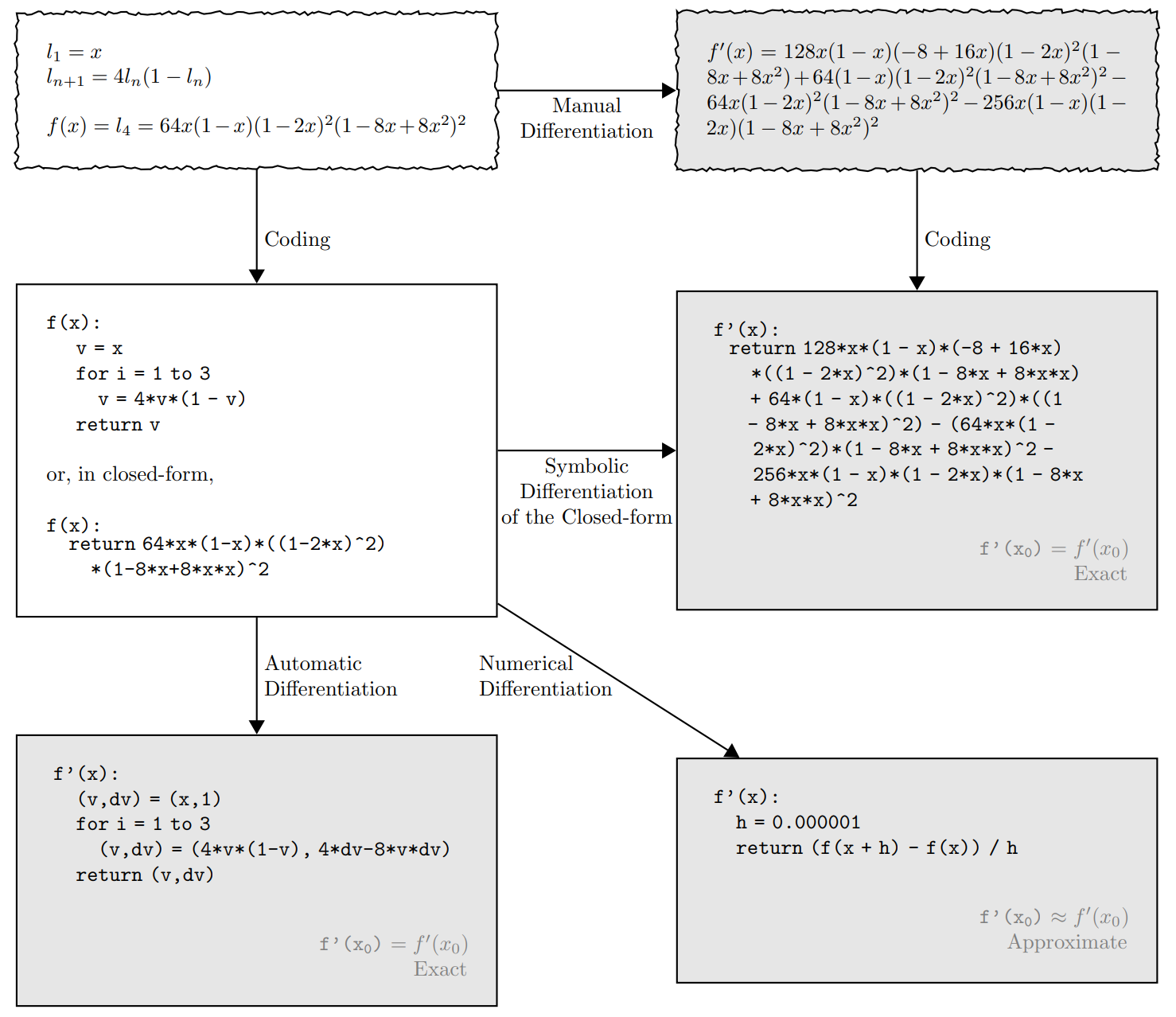
Analytical differentiation

$$ \frac{dz_{n+1}}{dx} = x\cos(z_n x)\frac{dz_n}{dx} + z_n\cos(z_n x) + 1,\quad \frac{dz_0}{dx}=0 $$

Even though the definition looks innocent, the full solution is very long. How about more complex models?

Numerical differentiation

For example, central difference: $$ f'(x) = \frac{f(x+h)-f(x-h)}{2h} + O(h^2) $$

Issues:

• Numerically unstable
  • Resolved by the complex step method, see HW3
• Slow if $f$ is expensive/high-dimensional

Alternatively - Complex Step

If a real-valued function $f(x)$ is analytic, then we can do analytic continuation to extend it to complex plane $f(x+iy)$.

Then, if we want the derivative at $x=x_0$ $$ f(x_0+ih) = f(x_0) + ih f'(x_0) - \frac{h^2}{2}f''(x_0) - i\frac{h^3}{6}f'''(x_0) $$

This gives us the complex step method: $$ f'(x_0) = \frac{\mathrm{imag}(f(x_0+ih))}{h} + O(h^2) $$

Pros:

• It looks like first-order finite difference, but it is second-order accurate
• Numerically stable

Cons:

• However, even slower then FD, as complex numbers are more expensive to work with
• Some functions do not support analytic continuation

Ref: Cleve Moler's blog

f = plt.figure(figsize=(6,4))
plt.loglog(ds, es[0], 'b-', label='Central Diff.')
plt.loglog(ds, es[1], 'r--', label='Complex Step')
_=plt.legend()
_=plt.xlabel('Step size')
_=plt.ylabel('Error')

Forward Mode

Or "Tangent" mode, think about the chain rule in differential form: $$ dy = \frac{dy}{dw_n}\left(\cdots\left(\frac{dw_2}{dw_1}\left(\frac{dw_1}{dx}dx\right)\right)\right) $$ for $y=w_n(\cdots (w_2(w_1(x))))$

Write out the first iteration step by step: $$ \begin{array}{cclcccl} x &=& ? \\ a &=& z_0 x \\ b &=& \sin(a) \\ z_1 &=& b+x \end{array} $$ Also try drawing in the form of computational graph.

Then, starting from the input, differentiate each step: $$ \begin{array}{cclcccl} x &=& ? &\Rightarrow& dx &=& ? \\ a &=& z_0 x &\quad& da &=& z_0 dx \\ b &=& \sin(a) &\quad& db &=& \cos(a)da \\ z_1 &=& b+x &\quad& dz_1 &=& db+dx \end{array} $$

Let the seed $dx=1$, $$ dz_1 = \frac{dz_1}{dx} = \frac{db}{dx}+1 = z_0\cos(z_0x)+1 $$

For multiple iterations: $$ \begin{array}{cclcccl} x &=& ? &\Rightarrow& dx &=& ? \\ z_0 &=& ? &\ & dz_0 &=& 0 \\ z_1 &=& \sin(z_0 x) + x &\ & dz_1 &=& x\cos(z_0 x)dz_0 + (z_0\cos(z_0 x) + 1)dx = dx \\ z_2 &=& \sin(z_1 x) + x &\ & dz_2 &=& x\cos(z_1 x)dz_1 + (z_1\cos(z_1 x) + 1)dx \\ \vdots &=& \vdots &\ & \vdots &=& \vdots \\ z_{n+1} &=& \sin(z_n x) + x &\ & dz_{n+1} &=& x\cos(z_n x)dz_n + (z_n\cos(z_n x) + 1)dx \end{array} $$

One could let the seed $dx=1$ again and note that $dz_0=0$, then one can find the gradient along with the forward pass, i.e. the function evaluation.

def df_fw(x):
    _dz, _dx = 0.0, 1.0         ##### NEW: Initialize the seed
    _z = 0.0                    # OLD code
    for _i in range(20):        # OLD code
        ##### NEW: Evaluate differentials
        _dz = x*np.cos(x*_z)*_dz + (_z*np.cos(x*_z) + 1) * _dx
        _z = np.sin(x*_z) + x   # OLD code
    return _dz

f = plt.figure(figsize=(6,4))
xx = np.linspace(0.0, 1.5, 201)
plt.plot(xx, df_ag(xx), 'r--', linewidth=4.0, label='Autograd')
plt.plot(xx, df_fw(xx), 'b-',  label='Forward AD')
plt.plot(xx, df_cs(xx), 'k-.', label='Complex Step')
_=plt.legend()

Reverse Mode

Or "Adjoint" mode, think about the chain rule in operator form: $$ \frac{d}{dx} = \frac{dw_1}{dx}\left(\frac{dw_2}{dw_1}\left(\cdots\left(\frac{dy}{dw_{n}}\frac{d}{dy}\right)\right)\right) $$ for $y=w_n(\cdots (w_2(w_1(x))))$

Again, write out one iteration step by step: $$ \begin{array}{cclcccl} x &=& ? \\ a &=& z_0 x \\ b &=& \sin(a) \\ z_1 &=& b+x \end{array} $$ Recall the computational graph too.

This time we start from the output, i.e. the last step, for one iteration: $$ \begin{array}{cclcccl} x &=& ? &\quad& \dfrac{d}{dx} &=& \dfrac{da}{dx}\dfrac{d}{da} + \dfrac{dz_1}{dx}\dfrac{d}{dz_1} = z_0\dfrac{d}{da} + \dfrac{d}{dz_1} \\ a &=& z_0 x &\quad& \dfrac{d}{da} &=& \dfrac{db}{da}\dfrac{d}{db} = \cos(a)\dfrac{d}{db} \\ b &=& \sin(a) &\quad& \dfrac{d}{db} &=& \dfrac{dz_1}{db}\dfrac{d}{dz_1} = \dfrac{d}{dz_1} \\ z_1 &=& b+x &\Rightarrow& \dfrac{d}{dz_1} &=& ? \end{array} $$

Now we know the operator, $$ \dfrac{d}{dx} = z_0\dfrac{d}{da} + \dfrac{d}{dz_1} = z_0\cos(a)\dfrac{d}{dz_1} + \dfrac{d}{dz_1} $$

And we can apply $\dfrac{d}{dx}$ to $z_1$, and note that $\dfrac{dz_1}{dz_1}=1$ $$ \frac{dz_1}{dx} = z_0\cos(z_0x)+1 $$ This is as if we set a seed $dz_1=1$.

For multiple iterations: $$ \begin{array}{cclcccl} x &=& ? &\quad& \dfrac{d}{dx} &=& \dfrac{dz_1}{dx}\dfrac{d}{dz_1} + \cdots + \dfrac{dz_{n+1}}{dx}\dfrac{d}{dz_{n+1}} \\ z_0 &=& ? &\quad& \dfrac{d}{dz_0} &=& \dfrac{dz_1}{dz_0}\dfrac{d}{dz_1} = 0 \\ z_1 &=& \sin(z_0 x) + x &\quad& \dfrac{d}{dz_1} &=& \dfrac{dz_2}{dz_1}\dfrac{d}{dz_2} \\ \vdots &=& \vdots &\quad& \vdots &=& \vdots \\ z_n &=& \sin(z_{n-1} x) + x &\quad& \dfrac{d}{dz_n} &=& \dfrac{dz_{n+1}}{dz_n}\dfrac{d}{dz_{n+1}} = x\cos(z_n x)\dfrac{d}{dz_{n+1}} \\ z_{n+1} &=& \sin(z_n x) + x &\Rightarrow& \dfrac{d}{dz_{n+1}} &=& ? \end{array} $$

One could let the seed $dz_{n+1}=1$, then find the gradient in the reversed order of the forward pass.

def df_rv(x):
    _z = 0.0                    # OLD code
    _s = [_z]                   ##### NEW: A list to store the intermediate
                                #####      z's in the iteration
    for _i in range(20):        # OLD code
        _z = np.sin(x*_z) + x   # OLD code
        _s.append(_z)           ##### NEW: intermediate z's

    ##### NEW: Below is an entirely new "reverse" pass
    _dz = 1.0    # Initialize the seed
    _dx = 0.0
    for _i in range(-1,-21,-1):    # Reversely go through the loop
        _z  = _s[_i-1]
        _dx = _dx + (_z*np.cos(_z*x)+1) * _dz
        _dz = (x*np.cos(_z*x)) * _dz
    return _dx

f = plt.figure(figsize=(6,4))
xx = np.linspace(0.0, 1.5, 201)
plt.plot(xx, df_ag(xx), 'r--', linewidth=4.0, label='Autograd')
plt.plot(xx, df_rv(xx), 'b-',  label='Reverse AD')
plt.plot(xx, df_cs(xx), 'k-.', label='Complex Step')
_=plt.legend()

Multi-variate Case

Given a chain of functions, $\vx\in\bR^N$, $\vy\in\bR^M$ $$ \vy = \vF_n(\vF_{n-1}(\cdots \vF_2(\vF_1(\vx)))) $$

The Jacobian is $$ \vJ = \ppf{\vy}{\vx} = \ppf{\vF_n}{\vF_{n-1}}\ppf{\vF_{n-1}}{\vF_{n-2}} \cdots \ppf{\vF_2}{\vF_{1}} \ppf{\vF_1}{\vx} $$

Next we consider the products of Jacobians and vectors, where we want to avoid products of Jacobians, because they are expensive.

Consider a Jacobian-Vector Product (JVP) $$ \vJ d\vx = \ppf{\vy}{\vx}d\vx = \left(\ppf{\vF_n}{\vF_{n-1}} \cdots \left(\ppf{\vF_2}{\vF_{1}} \left(\ppf{\vF_1}{\vx}d\vx \right)\right)\right) $$ Replace $d\vx=\ve_i$, where $\ve_i\in\bR^N$, the $i$th column of an identity matrix, $$ \vJ\ve_i = \left(\ppf{\vF_n}{\vF_{n-1}} \cdots \left(\ppf{\vF_2}{\vF_{1}} \left(\ppf{\vF_1}{\vx}\ve_i \right)\right)\right) $$ Then $\ve_i$ is like the seed, and one gets the $i$th column of $\vJ$, $$ \vJ\ve_i = \begin{bmatrix} \ppf{y_1}{x_i} \\ \ppf{y_2}{x_i} \\ \vdots \\ \ppf{y_M}{x_i} \end{bmatrix} $$ This is the Forward mode, good for fewer inputs than outputs.

Consider a Vector-Jacobian Product (VJP) $$ d\vy^T\vJ = d\vy^T\ppf{\vy}{\vx} = \left(\left(\left( d\vy^T\ppf{\vF_n}{\vF_{n-1}}\right) \ppf{\vF_{n-1}}{\vF_{n-2}}\right) \cdots \ppf{\vF_1}{\vx} \right) $$ Replace $d\vy=\ve_j$, where $\ve_j\in\bR^M$, the $j$th column of an identity matrix, $$ \ve_j^T\vJ = \left(\left(\left( \ve_j^T\ppf{\vF_n}{\vF_{n-1}}\right) \ppf{\vF_{n-1}}{\vF_{n-2}}\right) \cdots \ppf{\vF_1}{\vx} \right) $$ Then $\ve_j$ is like the seed, and one gets the $j$th row of $\vJ$, $$ \ve_j^T\vJ = \begin{bmatrix} \ppf{y_j}{x_1} & \ppf{y_j}{x_2} & \cdots & \ppf{y_j}{x_N} \end{bmatrix} $$ This is the Reverse mode, good for more inputs than outputs.

Comparison

Forward mode:

• Good for fewer inputs than outputs.
• Do not need to store intermediate results.

Reverse mode:

• Good for more inputs than outputs.
• Need to store the results and the "flow" of computation.

There is also Mixed mode.

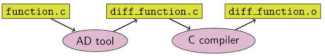
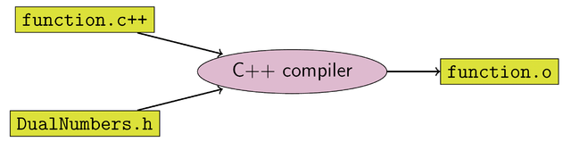
A bit about Implementation

• Source code transformation (SCT)

• Operator Overloading (OO) (e.g. dual number)

How about matrix functions?

det, log, exp, etc.

• Mature ML packages provide these.
• Otherwise, try this website: https://www.matrixcalculus.org/

How about Implicit functions?

Not unusual - e.g., a Newton solve for $x$, $f(x,b)=x^TAx-b=0$, given $b$

x = minimize(f, x0=init_guess)

Use implicit function theorem $$ \frac{\partial x}{\partial b} = \left(\frac{\partial f}{\partial x}\right)^{-1} \frac{\partial f}{\partial b} $$

More in Part II of Automatic Differentiation

How about Non-differentiable functions?

Not unusual as well - e.g., an argmax function

• Use its smoothed version, e.g., argmax --> softmax
• Use a probability distribution to "mollify" the discontinuity
• "Zeroth"-order optimization - estimate gradients by sampling

More in Part III of Automatic Differentiation

Back Propagation of Neural Networks

• Essentially reverse mode AD

Why Reverse instead of Forward?

• Denote $x,h,\theta$ is the input, output, and parameter of a layer.
• It is non-trivial to derive the gradient of loss w.r.t. parameters in intermediate layers

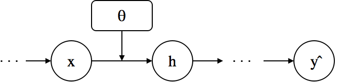
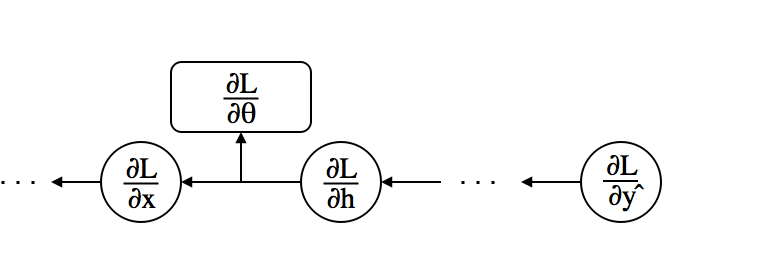
Idea of Back-Propagation

• Assuming that $\ppf{\cL}{h}$ is given, use the chain rule to compute the gradients $$\ppf{\cL}{\theta}=\underbrace{\ppf{\cL}{h}}_{\mbox{given}} \underbrace{\ppf{h}{\theta}}_{\mbox{easy}} \mbox{ , } \ppf{\cL}{x}=\underbrace{\ppf{\cL}{h}}_{\mbox{given}} \underbrace{\ppf{h}{x}}_{\mbox{easy}}$$
• We need only $\ppf{\cL}{\theta}$ for gradient descent. Why compute $\ppf{\cL}{x}$?
  • The previous layer needs it because $x$ is the output of the previous layer.

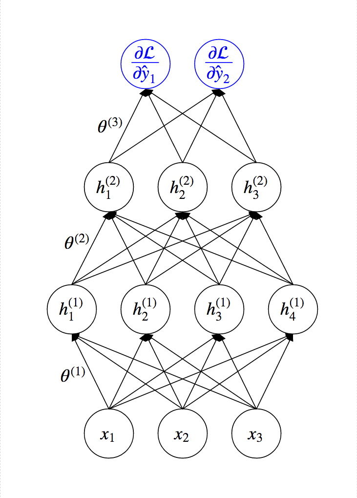
Idea of Back-Propagation

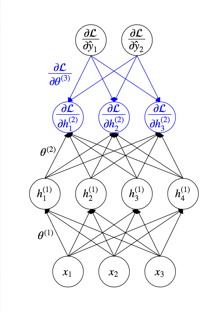
Idea of Back-Propagation

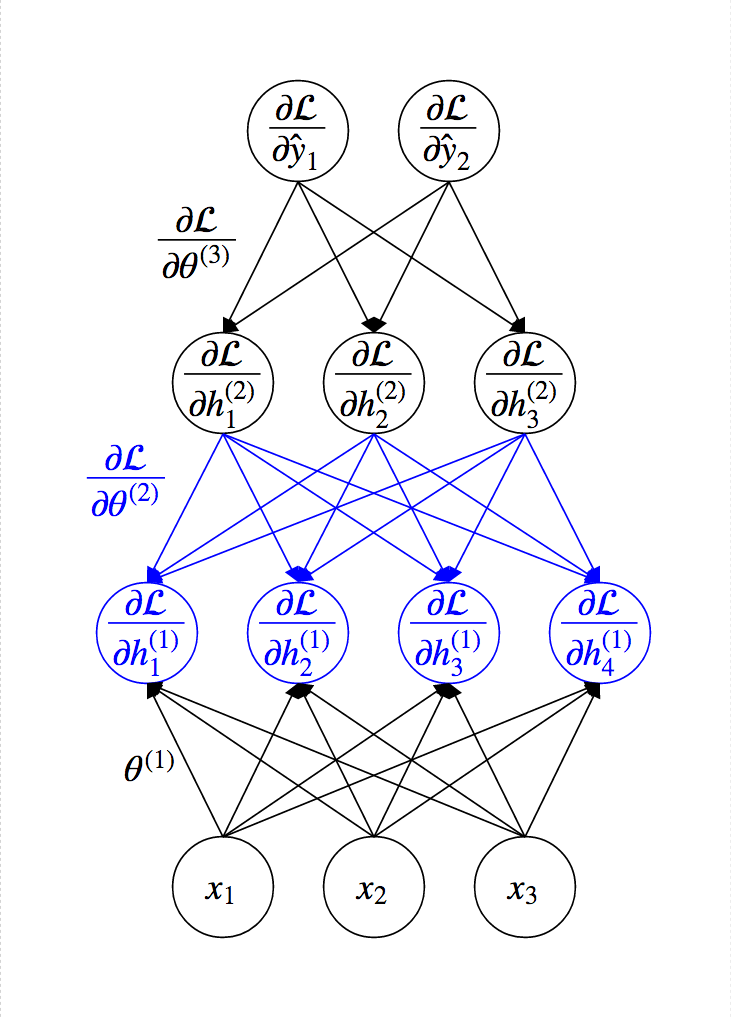
Idea of Back-Propagation

Idea of Back-Propagation

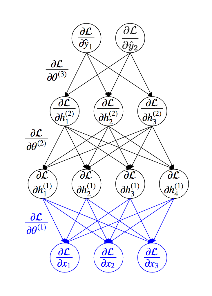
Back-Propagation Algorithm

• Compute $\ppf{\cL}{\vy}=\left[\ppf{\cL}{y_1}, \cdots, \ppf{\cL}{y_n}\right]^T$ directly from the loss function.
• For each layer (from top to bottom) with output $\vh$, input $\vx$, and weights $\vW$,
  • Assuming that $\ppf{\vh}{\cL}$ is given, compute gradients using the chain rule as follows: $$ \begin{align} \ppf{\cL}{\vW} &= \ppf{\cL}{\vh}\ppf{\vh}{\vW} \\ \ppf{\cL}{\vx} &= \ppf{\cL}{\vh}\ppf{\vh}{\vx} \end{align} $$

Practice: Linear

• Forward: $h_i=\sum_{j}w_{ij}x_j + b_i \iff \textbf{h} = \textbf{W}\textbf{x} + \textbf{b}$

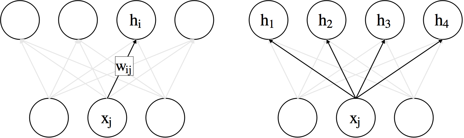
• Gradient w.r.t. parameters $$ \frac{\partial \mathcal{L}}{\partial w_{ij}} = \frac{\partial \mathcal{L}}{\partial h_{i}}\frac{\partial h_i}{\partial w_{ij}}=\frac{\partial \mathcal{L}}{\partial h_{i}}x_j \iff \ppf{\cL}{\vW} = \ppf{\cL}{\vh}\textbf{x}^{\top}$$ $$ \ppf{\cL}{\vb} = \ppf{\cL}{\vh} $$
• Gradient w.r.t. inputs $$ \frac{\partial \mathcal{L}}{\partial x_{j}} = \sum_{i} \frac{\partial \mathcal{L}}{\partial h_{i}}\frac{\partial h_i}{\partial x_{j}}=\sum_{i} \frac{\partial \mathcal{L}}{\partial h_{i}}w_{ij} \iff \ppf{\cL}{\vx} = \vW^{\top}\ppf{\cL}{\vh} $$

Practice: Non-Linear Activation (Sigmoid)

• Forward: $ h_i=\sigma (x_i) = \dfrac{1}{1+\exp\left(-x_i\right)} \iff \textbf{h} = \sigma \left(\textbf{x} \right) $

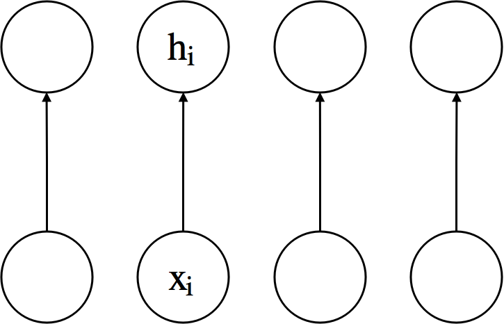
• Gradient w.r.t. inputs $$ \frac{\partial \mathcal{L}}{\partial x_{i}} = \frac{\partial \mathcal{L}}{\partial h_{i}}\frac{\partial h_i}{\partial x_{i}}=\frac{\partial \mathcal{L}}{\partial h_{i}}\sigma(x_i)(1-\sigma(x_i))=\frac{\partial \mathcal{L}}{\partial h_{i}}h_i(1-h_i)$$ $$ \ppf{\cL}{\vx}=\ppf{\cL}{\vh} \odot \vh \odot (\textbf{1} - \vh) $$