$$ \newcommand\ddf[2]{\dfrac{\mathrm{d} #1}{\mathrm{d} #2}} \newcommand\ppf[2]{\dfrac{\partial #1}{\partial #2}} \newcommand{\bE}{\mathbb{E}} \newcommand{\cE}{\mathcal{E}} \newcommand{\cF}{\mathcal{F}} \newcommand{\cJ}{\mathcal{J}} \newcommand{\cL}{\mathcal{L}} \newcommand{\cM}{\mathcal{M}} \newcommand{\cN}{\mathcal{N}} \newcommand{\cR}{\mathcal{R}} \newcommand{\cU}{\mathcal{U}} \newcommand{\vA}{\mathbf{A}} \newcommand{\vI}{\mathbf{I}} \newcommand{\vK}{\mathbf{K}} \newcommand{\vM}{\mathbf{M}} \newcommand{\vQ}{\mathbf{Q}} \newcommand{\vR}{\mathbf{R}} \newcommand{\vU}{\mathbf{U}} \newcommand{\vb}{\mathbf{b}} \newcommand{\vc}{\mathbf{c}} \newcommand{\vd}{\mathbf{d}} \newcommand{\vf}{\mathbf{f}} \newcommand{\vg}{\mathbf{g}} \newcommand{\vm}{\mathbf{m}} \newcommand{\vu}{\mathbf{u}} \newcommand{\vw}{\mathbf{w}} \newcommand{\vtt}{\boldsymbol{\theta}} \newcommand{\vtvt}{\boldsymbol{\vartheta}} \newcommand{\vtl}{\boldsymbol{\lambda}} \newcommand{\vtf}{\boldsymbol{\phi}} \newcommand{\vty}{\boldsymbol{\psi}} $$
Motivation
Previously ...
a Newton solve for $x$, $f(x,b)=x^8-x^2-b=0$, given $b$
- Implicit, because we cannot write $x$ as an analytical function of $b$.
an
argmaxfunction, e.g., $x=\mathrm{arg max} f(x)$- Non-differentiable, because an infinitesimal change in $f$ can result in large, finite change in $x$.
How to backprop these functions?
But before that, when do we need to deal with these?
Example 1: All models are wrong, but some are useful.
- In traditional computational analysis, the physics cannot be precisely captured
- e.g., turbulence closure, constitutive relation modeling
- Uncertainty in prediction/design $\rightarrow$ Large safety factor and performance penalty
- ML can be mebedded into traditional analysis for better predictive capability.
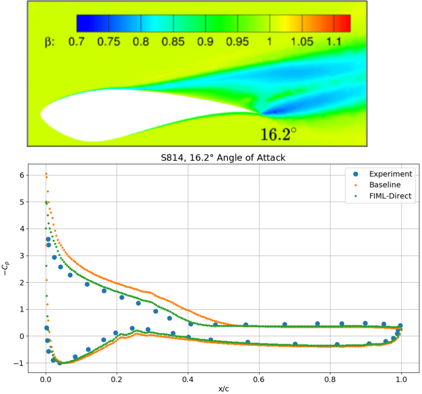 (Figure from Holland, Baeder etc. 2019)
Example 2: Don't learn what you already know
- Some ML tasks involves steps that can be done by traditional analysis
- e.g., path planning and trajectory tracking in robotics
- Replacing these steps by pure NN's takes extra effort and usually does not extrapolate well
- Traditional analysis can be embedded into ML for better generalizability and robustness.
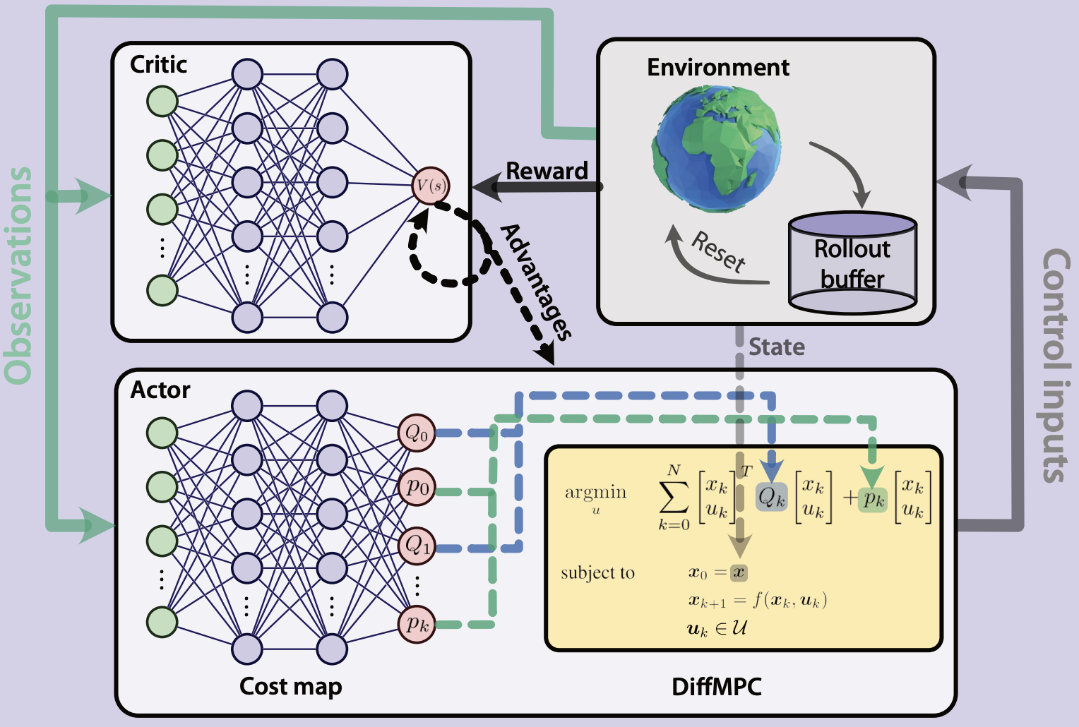
[1] Romero et al. Actor-Critic Model Predictive Control: Differentiable Optimization meets Reinforcement Learning. 2023.
Posing the Problem
From an NN perspective, a model problem is
$$ \boxed{\text{Given }\vtt}\rightarrow \boxed{\text{Solve }\min_{\vu} \cE(\vu;\vtt)\text{ or }\arg\min_{\vu} \cE(\vu;\vtt)}\rightarrow \boxed{\text{Compute }\cJ(\vu;\vtt)} $$
- $\vtt$ is the learnable parameter and $\cJ$ is the loss
- The middle step is an optimization of an implicit function $\cE$
- Let's see some examples next
Example 1: Model Calibration
Consider a solid mechanics problem. The solution is found by minimizing energy $$ \cE(\vu) = \vu^\top\vK\vu + \vf^\top\vu $$ where $\vu$ is displacement and $\vf$ is load.
- But now the stiffness matrix $\vK$ is not fully known, so we assume $\vK=\vK_0+\delta\vK_{NN}(\vtt)$ and denote $\cE(\vu;\vtt)$.
- Given data set $\{(\vf_i,\vu_i)\}_{i=1}^N$ we want to learn $\delta\vK_{NN}$.
Formally we can write it as a nested optimization problem, $$ \begin{align} \min_{\vtt} &\quad \cJ(\hat{\vu};\vtt) = \sum_{i=1}^N \lVert\vu_i-\hat{\vu}_i\rVert^2 \\ \mathrm{s.t.} &\quad \min_{\vu} \cE(\hat{\vu}_i;\vtt) = \hat{\vu}_i^\top(\vK_0+\vK_{NN}(\vtt))\hat{\vu}_i + \vf_i^\top\hat{\vu}_i,\quad i=1,2,\cdots,N \end{align} $$ ... and the computation graph is what we have shown earlier.
The same idea applies to many other scenarios, e.g.,
- Fluid dynamics:
- $\min\cE(\vu)$ solves Navier-Stokes equation, $\vu$ - density, momentum, energy
- $\cJ$ to minimize difference in simulation vs. experiment for, e.g., pressure data on an airfoil
- $\min\cE(\vu;\vtt)$ with correction in turbulence production term in the fluid solver
- System dynamics:
- $\min\cE(\vu)$ solves flight dynamics equation, $\vu$ - linear & angular displacement/velocity
- $\cJ$ to minimize difference in sim. vs. exp. for, e.g., dynamical response
- $\min\cE(\vu;\vtt)$ with correction in unknown external forcing term
Example 2: Imitation Learning
Consider a model predictive controller (MPC). $$ \begin{align} \min_{\vu,\vf} &\quad \cE(\vu;\vtt) = \sum_{i=1}^N (\vu_i-\vu_{r,i})^\top\vQ(\vu_i-\vu_{r,i}) + \vf_i^\top\vR\vf_i \\ \mathrm{s.t.} &\quad \vu_{i+1}=\vg(\vu_i,\vf_i),\quad i=1,2,\cdots,N-1 \end{align} $$ with states $\vu$, inputs $\vf$, and dynamics $\vg$; $\vu_r$ is the trajectory to track.
- In practice, the choice of $\vQ$ and $\vR$ may require extensive tuning.
- Given data set of "expert demonstrations" (e.g., by human) for optimal inputs $\{\vf_i\}_{i=1}^N$ and states $\{\vu_i\}_{i=1}^N$.
- How to learn $\vtt=[\vQ,\vR]$ from the dataset?
This is again a nested optimization problem,
$$ \begin{align} \min_{\vtt} &\quad \cJ(\hat{\vu},\hat{\vf};\vtt) = \sum_{i=1}^N \lVert\vu_i-\hat{\vu}_i\rVert^2 + \lVert\vf_i-\hat{\vf}_i\rVert^2 \\ \mathrm{s.t.} &\quad \min_{\hat{\vu},\hat{\vf}} \ \cE(\hat{\vu};\vtt) = \sum_{i=1}^N (\hat{\vu}_i-\vu_{r,i})^\top\vQ(\hat{\vu}_i-\vu_{r,i}) + \hat{\vf}_i^\top\vR\hat{\vf}_i \\ &\quad \ \mathrm{s.t.}\quad \hat{\vu}_{i+1}=\vg(\hat{\vu}_i,\hat{\vf}_i),\quad i=1,2,\cdots,N-1 \end{align} $$
... just that we got some constraints in the inner problem.
General Form of Problem
The above examples suggest the following general form to tackle: $$ \begin{align} \min_{\vtt} &\quad \cJ(\vu;\vtt) \\ \mathrm{s.t.} &\quad \min \cE(\vu;\vtt) \\ &\quad \mathrm{s.t.} \quad \vc(\vu;\vtt) = 0 \end{align} $$
- $\cJ$: The outer objective - typically the loss for learning
- $\cE$ and $\vc$: The inner objective and constraints
- The inner optimization problem
- Implicitly define $\vu$ as a function of $\vtt$
- Inequality constraints can be added too
For the purpose of ML, we still want $\ddf{\cJ}{\vtt}$.
Strategies for BP
Two cases for the inner problem:
- Non-differentiable, or a black box
- e.g., sampling-based, or an external solver not in a learning framework
- The rest (easier) case
- This typically means the evaluation of $\cE$ and $\vc$ can be backproped
Easier Case First
Since all the terms are differentiable, consider the equivalent form by Lagrangian multiplier, $$ L_i(\vu,\vtl;\vtt) = \cE(\vu;\vtt) + \vtl^\top \vc(\vu;\vtt) $$ The necessary condition for optimality is $$ \ppf{L_i}{\vu} = 0,\quad \ppf{L_i}{\vtl} = 0 $$ So solving the inner problem is equivalent to solving the above nonlinear algebraic equations. Denote as $$ \cR(\vu;\vtt) = 0 $$ (dropping $\vtl$ for conciseness)
The inner problem is then solved by, e.g., Newton iterations
- Starting from initial guess $$ \vu^{(0)},\quad \cR^{(0)} = \cR(\vu^{(0)};\vtt) $$
- Iterate $$ \vu^{(k+1)} = \vu^{(k)} - (\nabla_{\vu}\cR^{(k)})^{-1} \cR^{(k)} $$
- Until convergence, e.g., $$ \lVert \vu^{(n)}-\vu^{(n-1)} \rVert \leq \epsilon $$
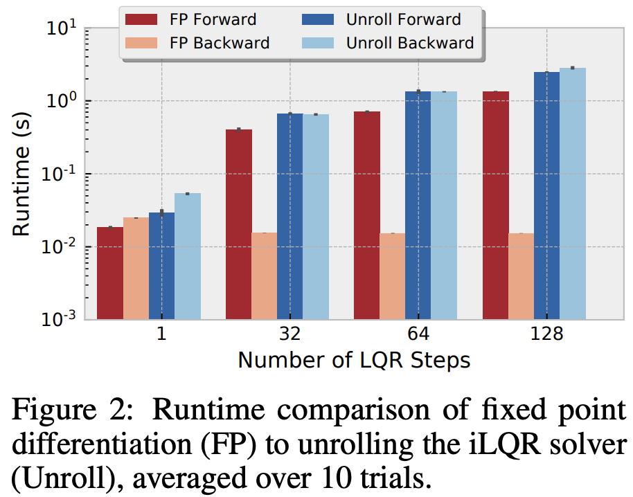
Brutal force: Unrolling
While the inner problem is an implicit function, the iterations are explicit. $$ \boxed{\vu^{(0)}; \vtt} \rightarrow \boxed{\cR^{(0)}} \rightarrow \boxed{\vu^{(1)} = \vu^{(0)} - (\nabla_{\vu}\cR^{(0)})^{-1} \cR^{(0)}} \rightarrow \boxed{\vu^{(2)} = \vu^{(1)} - ...} \rightarrow \boxed{...} \rightarrow \boxed{\vu=\vu^{n}} $$ We can unroll and BP the entire iteration process - each iteration is effectively one layer.
- Pros: Easy to implement - as long as the iterations are implemented in a ML package, the package can do BP for you
- Cons: Slow - need to BP through all iterations (similar to LSTM)
Unrolling - a fix
The initial guess is free to choose, and what if it is exactly the solution? How about:
First a regular solve, but do not retain gradients $$ \boxed{\vu^{(0)}; \vtt} \rightarrow \boxed{\cR^{(0)}} \rightarrow \boxed{\vu^{(1)} = \vu^{(0)} - (\nabla_{\vu}\cR^{(0)})^{-1} \cR^{(0)}} \rightarrow \boxed{\vu^{(2)} = \vu^{(1)} - ...} \rightarrow \boxed{...} \rightarrow \boxed{\vu=\vu^{n}} $$ Then use $\vu^{n}$ as the initial guess and "pretend" to solve the problem in one iteration; retain gradients here $$ \boxed{\vu^{(n)}; \vtt} \rightarrow \boxed{\cR^{(n)}} \rightarrow \boxed{\vu^{(n+1)} = \vu^{(n)} - (\nabla_{\vu}\cR^{(n)})^{-1} \cR^{(n)}} \rightarrow \boxed{\vu=\vu^{n+1}} $$ BP the second round only
- Pros: Barely any more effort to implement, and much faster
- Cons: Could still be slow, as the BP does not leverage problem structure
- e.g., BP through a linear solve $\nabla_{\vu}\cR^{(n)}$, which can be expensive
(Possibly) Better solution: Adjoint
To be discussed in a minute.
- Pros: Fast and accurate
- Cons: Takes time to implement
Non-differentiable Case
Essentially, one can only do forward evaluation for the inner problem, i.e.,
- A function that computes $\vu$ given $\vtt$. Denote $\vu=\cF_{ND}(\vtt)$
- Rewrite the nested problem as $$ \min_\vtt \cJ(\cF_{ND}(\vtt),\vtt) $$
Whenever possible, avoid getting trapped in this scenario. But if you have to deal with it...
Brutal force: Penalty/Surrogate
Define a surrogate NN to replace $\cF_{ND}$ to estimate $\vu$ $$ \hat{\vu} = \cF_{NN}(\vtt;\vartheta) $$ Learn the original model and the surrogate simultaneously with two losses $$ \min_{\vtt,\vartheta} \cJ(\hat{\vu},\vtt) + \lVert \cF_{NN}(\vtt;\vartheta) - \cF_{ND}(\vtt) \rVert^2 $$ $\cF_{ND}(\vtt)$ is used as if a dataset generated on the fly
- Pros: Easy to implement; (typically) fast to evaluate in prediction
- Cons: Additional computational cost; $\cF_{NN}$ can be hard to train; only weak enforcement of $\cF_{ND}$ in prediction
(Possibly) Better solution: Probabilistic formulation
To be discussed in a minute.
- Pros: Opposite of the previous cons
- Cons: Effective only for low-dim $\vtt$
Recap
Next we will discuss two methods for BP implicit functions:
- Adjoint method for differentiable cases
- Probabilistic method for non-differentiable cases
Adjoint Method for Differentiable Cases
Consider the optimization problem in general, $$ \begin{align} \min_{\vtt} &\quad \cJ(\vu;\vtt) \\ \mathrm{s.t.} &\quad \cR(\vu;\vtt) = 0 \end{align} $$ where $\cR(\vu;\vtt)=0$ represents the inner problem.
Formulation by adjoint variables
For optimization, one wants the full derivative of $\cJ(\vu;\vtt)$ w.r.t. $\vtt$, i.e. $$ \ddf{\cJ(\vu;\vtt)}{\vtt} = \ppf{\cJ}{\vu}\ppf{\vu}{\vtt} + \ppf{\cJ}{\vtt} $$ where $\ppf{\vu}{\vtt}$ is non-trivial to compute.
From the constraint, one knows, $$ \ddf{\cR(\vu;\vtt)}{\vtt} = \ppf{\cR}{\vu}\ppf{\vu}{\vtt} + \ppf{\cR}{\vtt} = 0 $$ or $$ \ppf{\vu}{\vtt} = \left(-\ppf{\cR}{\vu}\right)^{-1}\ppf{\cR}{\vtt} $$
Therefore, $$ \ddf{\cJ(\vu;\vtt)}{\vtt} = \ppf{\cJ}{\vu}\left(-\ppf{\cR}{\vu}\right)^{-1}\ppf{\cR}{\vtt} + \ppf{\cJ}{\vtt} $$
Now let $$ \vtf^T = -\ppf{\cJ}{\vu}\left(\ppf{\cR}{\vu}\right)^{-1} $$ or $$ \left(\ppf{\cR}{\vu}\right)^T\vtf = -\left(\ppf{\cJ}{\vu}\right)^T $$
This last equation is called the Adjoint Equation, and $\vtf$ is called the Adjoint Variable.
As a result, the full derivate of $\cJ(\vu;\vtt)$ w.r.t. $\vtt$ is computed as follows,
- Given $\vtt$, solve $\cR(\vu;\vtt)=0$ to find $\vu$
- In this process one obtains $\ppf{\cR}{\vu}$.
- Given $\vtt$ and $\vu$, find $\ppf{\cJ}{\vu}$, $\ppf{\cJ}{\vtt}$, and $\ppf{\cR}{\vtt}$.
- Solve the adjoint equation and find $\vtf$. $$ \left(\ppf{\cR}{\vu}\right)^T\vtf = -\left(\ppf{\cJ}{\vu}\right)^T $$
- The gradient of $\cJ$ $$ \ddf{\cJ(\vu;\vtt)}{\vtt} = \vtf^T\ppf{\cR}{\vtt} + \ppf{\cJ}{\vtt} $$
Alternative: Formulation by Lagrange multipliers
Introduce a vector of Lagrange multipliers $\vtf$ $$ \cL(\vu;\vtt) = \cJ(\vu;\vtt) + \vtf^T \cR(\vu;\vtt) $$
Now one wants the full derivative of $\cL(\vu;\vtt)$ w.r.t. $\vtt$, i.e. $$ \ddf{\cL(\vu;\vtt)}{\vtt} = \ppf{\cJ}{\vu}\ppf{\vu}{\vtt} + \ppf{\cJ}{\vtt} + \vtf^T\left( \ppf{\cR}{\vu}\ppf{\vu}{\vtt} + \ppf{\cR}{\vtt} \right) $$
The RHS is $$ \ppf{\cJ}{\vtt} + \vtf^T\ppf{\cR}{\vtt} + \left(\ppf{\cJ}{\vu} + \vtf^T\ppf{\cR}{\vu}\right)\ppf{\vu}{\vtt} $$
One can eliminate $\ppf{\vu}{\vtt}$ by setting the bracket to zero, $$ \ppf{\cJ}{\vu} + \vtf^T\ppf{\cR}{\vu} = 0 $$ or the adjoint equation $$ \left(\ppf{\cR}{\vu}\right)^T\vtf = -\left(\ppf{\cJ}{\vu}\right)^T $$
Extra: Multiple inner problems
It is not uncommon if a ML model involves multiple implicit functions. The optimization problem becomes $$ \begin{align} \min_{\vtt} &\quad \cJ(\vU;\vtt) \\ \mathrm{s.t.} &\quad \cR_j(\vU;\vtt) = 0,\quad j=1,\cdots,m \end{align} $$ where $m$ inner problems are involved, with unknowns $\vU=\{\vu_1,\cdots,\vu_m\}$.
Introduce a set of Lagrange multipliers, or the adjoint variables, $$ \cL(\vU;\vtt) = \cJ(\vU;\vtt) + \sum_{j=1}^m \vtf_j^T \cR_j(\vU;\vtt) $$
Take the full derivative, $$ \begin{align} \ddf{\cL(\vu;\vtt)}{\vtt} &= \ppf{\cJ}{\vU}\ppf{\vU}{\vtt} + \ppf{\cJ}{\vtt} + \sum_{j=1}^m \vtf_j^T\left( \ppf{\cR_j}{\vU}\ppf{\vU}{\vtt} + \ppf{\cR_j}{\vtt} \right) \\ &= \ppf{\cJ}{\vtt} + \sum_{j=1}^m \vtf_j^T\ppf{\cR_j}{\vtt} + \sum_{j=1}^m \left(\vtf_j^T\ppf{\cR_j}{\vU} + \ppf{\cJ}{\vU}\right)\ppf{\vU}{\vtt} \end{align} $$
A set of $m$ coupled adjoint equations is identified as $$ \sum_{j=1}^m \left(\ppf{\cR_j}{\vu_i}\right)^T\vtf_j = \left(\ppf{\cJ}{\vu_i}\right)^T,\quad i=1,\cdots,m $$
Numerical Example
We solve a 1D advection-diffusion equation for $x\in [0,1]$ $$ p u' - u'' = f(x;\vtt),\quad u(0)=u_0,\ u'(1)=n_1 $$ where $p$ is a constant, representing wave speed.
The RHS contains some unknown parameters $$ f(x;\vtt) = x^2 + \theta_1 x + \theta_2 $$
Suppose we know a solution $u^*$ found at the true parameters $\theta^*$. To infer $\theta^*$ from $u^*$, we solve $$ \begin{align*} \min_{\vtt} &\quad J(u;\vtt) \equiv \int_0^1 (u-u^*)^2 dx \\ \mathrm{s.t.} &\quad p u' - u'' = f(x;\vtt),\quad u(0)=u_0,\ u'(1)=n_1 \end{align*} $$
xx = np.linspace(0,1,41)
f = plt.figure(figsize=(6,4))
plt.plot(xx, fu(xx));

System Discretization
We use a generic Galerkin method to discretize the differential equation and the objective.
Specifically, we pick $N$ Legendre polynomials as basis functions, and represent the solution as $$ u(x) = \sum_{i=1}^N u_i\psi_i(x) \equiv \vty^T(x) \vu $$
f, ax = plt.subplots(ncols=2, figsize=(8,4))
for _i in range(0,5):
    ax[0].plot(xx, eval_leg0(_i, xx), label=f"Order={_i}")
    ax[1].plot(xx, eval_leg1(_i, xx))
ax[0].legend()
ax[0].set_title("Legendre polynomials")
ax[1].set_title("Derivatives");

The objective is converted to a quadratic form, $$ \cJ(\vu;\vtt) = \int_0^1 \left( \vty^T\vu - u^* \right)^2 dx \equiv \vu^T \vM \vu - 2\vu^T \vm + \text{const} $$ where $$ \vM = \int_0^1 \vty\vty^T dx,\quad \vm = \int_0^1 \vty u^* dx $$
The equation is converted to a linear system,
$$
\cR(\vu;\vtt) = \vA\vu - \vb(\vtt) = 0
$$
where for the formulation of $\vA$ see the Differential Equations slides in Math review, and
$$
\vb(\vtt) = \int_0^1 \vty f(x,\vtt) dx
$$
Adjoint-based Optimization
This brings us to the standard form: $$ \begin{align*} \min_{\vtt} &\quad \cJ(\vu;\vtt) \\ \mathrm{s.t.} &\quad \cR(\vu;\vtt) = 0 \end{align*} $$ Now suppose we start with an initial guess, say $\vtt^{(0)}=[10.0, 10.0]$.
Then, to use the adjoint formulation to obtain the gradients for optimization $\ddf{\cL(\vu;\vtt)}{\vtt}$ at $\vtt^{(0)}$ -
First, we solve $\vu^{(0)}$ at $\vtt^{(0)}$. Clearly this is totally off.
theta0 = [10.0, 10.0]
sol, mats = galerkin(M, N, p, ub, nb, theta0)
print(obj(sol)[0])
compare_sol(sol, fu, 41);
0.6717431265076316

Then, we solve the adjoint problem $$ \left(\ppf{\cR}{\vu}\right)^T\vtf = -\left(\ppf{\cJ}{\vu}\right)^T $$ where $\ppf{\cR}{\vu}=\vA$, $\ppf{\cJ}{\vu}=(2\vM\vu-2\vm)^T$
And evaluate the gradients $$ \ddf{\cL(\vu;\vtt)}{\vtt} = \ppf{\cJ}{\vtt} + \vtf^T \ppf{\cR}{\vtt} $$ where $\ppf{\cJ}{\vtt}=0$ and $\ppf{\cR}{\vtt}=-\ppf{\vb}{\vtt}$
Adjoint-based gradients, verified by finite difference:
# Adjoint
sol, mats = galerkin(M, N, p, ub, nb, theta0)  # Forward solve
_, gda = galerkin_da(sol, mats, obj)           # Adjoint/Backward solve
# Finite difference, using a SciPy function
def Jfd(qs):
    sol, _ = galerkin(M, N, p, ub, nb, qs)
    d, _ = obj(sol)
    return d
gfd = approx_fprime(theta0, Jfd)

print(f"Adjoint: {gda}, FD: {gfd}")
Adjoint: [0.04238442 0.09196361], FD: [0.04238444 0.0919636 ]
Now let's use a vanilla optimizer from SciPy to solve the problem (i.e., train the model)
def Jda(qs):
    sol, mats = galerkin(M, N, p, ub, nb, qs)
    fun, grd = galerkin_da(sol, mats, obj)
    return fun, grd
res = minimize(Jda, theta0, method="l-bfgs-b", jac=True)
print(res)
  message: CONVERGENCE: NORM_OF_PROJECTED_GRADIENT_<=_PGTOL
  success: True
   status: 0
      fun: 7.840073109219852e-09
        x: [ 3.404e-04 -2.283e-04]
      nit: 4
      jac: [-2.017e-08 -4.432e-08]
     nfev: 8
     njev: 8
 hess_inv: <2x2 LbfgsInvHessProduct with dtype=float64>
# Check the converged solutions, i.e., "learned" model
sol, mats = galerkin(M, N, p, ub, nb, res.x)
compare_sol(sol, fu, 41);

# Note that much more cost would be incurred if we optimize
# by BRUTAL force (i.e., finite difference)
res = minimize(Jfd, theta0, method="l-bfgs-b", jac=False)
print(res)  # Look at `nfev`: function evaluation
  message: CONVERGENCE: NORM_OF_PROJECTED_GRADIENT_<=_PGTOL
  success: True
   status: 0
      fun: 7.84006204764976e-09
        x: [ 4.063e-04 -2.550e-04]
      nit: 4
      jac: [-7.499e-09 -2.315e-08]
     nfev: 24
     njev: 8
 hess_inv: <2x2 LbfgsInvHessProduct with dtype=float64>
Key take-away: Adjoint formulation enables machine learning with large scale simulations.
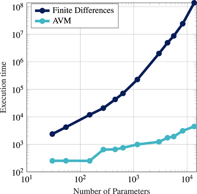
[Left] Neustock et al. Nature 2019; [Right] Amos et al. NeurIPS 2018
Probabilistic Method for Non-Differentiable Cases
Recall now the problem has to be written as $$ \min_\vtt \cJ(\cF_{ND}(\vtt),\vtt) $$ where $\cF_{ND}$ might not be differentiable.
We assume scalar $\cF$ here.
Next we present two routes for finding the equivalent or approximate quantities to $$ \ppf{\cF_{ND}(\vtt)}{\vtt}\text{, or in short, }\nabla_\vtt\cF $$ so that we can work with non-differentiable functions in a differentiable framework.
Route 1: Zeroth-order Estimate
For differentiable cases, one can use finite difference to estimate gradients $$ (\nabla_\vtt \cF)\vw = \frac{\cF(\vtt+\epsilon\vw)-\cF(\vtt)}{\epsilon} + O(\epsilon),\quad \text{for sufficiently small }\epsilon $$ Looping over unit vectors $\vw=[1,0,\cdots,0],[0,1,\cdots,0]$, etc. gives the columns of $\nabla_\vtt \cF$
Now define a probabilistic generalization of the finite difference $$ \tilde{\nabla}_\vtt\cF = \bE_\vw\left[ \frac{\cF(\vtt+\epsilon\vw)-\cF(\vtt)}{\epsilon}\vw^\top \right],\quad \text{for small }\epsilon,\ \vw \sim \cN(0,\vI) $$
Does not require $\cF$ to be differentiable
Practically, we sample, say, $N$ $\vw_i$ from $\cN(0,\vI)$, and estimate $$ \tilde{\nabla}_\vtt\cF = \frac{1}{N} \sum_{i=1}^N \frac{\cF(\vtt+\epsilon\vw_i)-\cF(\vtt)}{\epsilon}\vw_i^\top $$
If $\cF$ were differentiable, $$ \cF(\vtt+\epsilon\vw) \approx \cF(\vtt) + \epsilon(\nabla_\vtt\cF)\vw $$ Then we recover finite difference when $\epsilon\rightarrow 0$ $$ \tilde{\nabla}_\vtt\cF = \bE_\vw\left[ \frac{\cF(\vtt+\epsilon\vw)-\cF(\vtt)}{\epsilon}\vw^\top \right] = \bE_\vw\left[ (\nabla_\vtt\cF)\vw\vw^\top \right] = (\nabla_\vtt\cF) \underbrace{\bE_\vw\left[ \vw\vw^\top \right]}_{=\vI} = \nabla_\vtt\cF $$
A discussion on variance
You might notice the probabilistic version could probably be simplified $$ \tilde{\nabla}_\vtt\cF = \bE_\vw\left[ \frac{\cF(\vtt+\epsilon\vw)-\cF(\vtt)}{\epsilon}\vw^\top \right] = \frac{1}{\epsilon}\bE_\vw\left[ \cF(\vtt+\epsilon\vw)\vw^\top \right] - \frac{1}{\epsilon}\bE_\vw\left[\cF(\vtt)\vw^\top \right] = \frac{1}{\epsilon}\bE_\vw\left[ \cF(\vtt+\epsilon\vw)\vw^\top \right] $$ because, in the second $\bE_\vw$, $\cF(\vtt)$ is independent of $\vw$ and $\bE[\vw]=0$ by definition.
Why people do not use this simpler version?
To quantify the quality of an estimation, we consider
- Bias: Average deviation of the mean from truth
- Non-zero bias gives erroneous gradients - bad for optimization
- Variance: Spread of deviation
- Higher variance gives larger randomness of gradients - bad for optimization
- Ideally we want zero bias and low variance
Both probabilistic versions are already zero bias, how about variance?
Consider a general case - find $b$ to minimize the variance of $$ \vg(b) = \frac{\cF(\vtt+\epsilon\vw)-b}{\epsilon}\vw $$ Already know $\bE_\vw[\vg(b)]=0$, so we only need $$ \min_b \lVert\bE_{\vw}[\vg\vg^\top]\rVert,\text{ or loosely: } \min_b \bE_{\vw}[\lVert\vg\rVert^2] $$
Note that the objective is simply a quadratic function of $b$ $$ \bE_{\vw}[\lVert\vg\rVert^2] = \bE_{\vw}\left[ \left(\frac{\cF(\vtt+\epsilon\vw)-b}{\epsilon}\right)^2 \lVert\vw\rVert^2 \right] = \frac{1}{\epsilon^2}\bE_{\vw}[\lVert\vw\rVert^2] b^2 + [blah] b + [blah] $$ so the minimizer can be found analytically $$ b^* = \frac{\bE_{\vw}[\cF(\vtt+\epsilon\vw)\lVert\vw\rVert^2]}{\bE_{\vw}[\lVert\vw\rVert^2]} $$ One can either estimate $b^*$ at each iteration, or simply choose $b^*\approx \cF(\vtt)$
- This brings back our initial probabilistic formulation!
Side Note
Along a similar vein, but a different route, one would get "Evolution Strategy" (ES) type algorithms for optimization.
- ES algorithms have decades of history of development. One popular variant is CMA-ES.
One notable instance of ES in ML is the following work from OpenAI:
- Salimans et al. Evolution Strategies as a Scalable Alternative to Reinforcement Learning. ArXiv 2017.
Route 2: Policy Gradient
Let's consider a special case, $$ \cF(\vtt) = \arg\max_\vu p(\vu;\vtt) $$ i.e., finding the $\vu$ that is "the most probable" in a probability distribution.
- Key idea: $\cF$ is non-differentiable, but $p$ is.
- This set up is common in reinforcement learning - $p$ is the "policy".
- We will return to the general case in the next route.
This route involves several transformations - First an approximate objective (using $\max$ for consistency) $$ \max_\vtt \cJ(\cF(\vtt))=\cJ(\arg\max_\vu p(\vu;\vtt)) \Rightarrow \max_\vtt \int_\vu \cJ(\vu)p(\vu;\vtt) d\vu $$
The new objective is differentiable $$ \nabla_\vtt \left( \int_\vu \cJ(\vu)p(\vu;\vtt) d\vu \right) = \int_\vu \cJ(\vu) \nabla_\vtt p(\vu;\vtt) d\vu $$
But it requires an expensive integral over $\vu$ - So we do the log-trick $$ RHS = \int_\vu \cJ(\vu) \left(\frac{\nabla_\vtt p(\vu;\vtt)}{p(\vu;\vtt)}\right)p(\vu;\vtt) d\vu = \int_\vu \cJ(\vu) \nabla_\vtt \log p(\vu;\vtt) p(\vu;\vtt) d\vu $$
Now the gradient can be written as an expectation - which can be estimated from $N$ samples $$ \nabla_\vtt \cJ \approx \bE_\vu[\cJ(\vu) \nabla_\vtt \log p(\vu;\vtt)] \approx \frac{1}{N}\sum_{i=1}^N \cJ(\vu_i) \nabla_\vtt \log p(\vu_i;\vtt) $$
Variance
Just like the previous route, here we can adjust the gradient estimation to reduce the variance.
First note that subtracting a constant does not change the estimation $$ \bE_\vu[(\cJ(\vu)-b) \nabla_\vtt \log p(\vu;\vtt)] = \bE_\vu[\cJ(\vu) \nabla_\vtt \log p(\vu;\vtt)] - b \underbrace{\bE_\vu[\nabla_\vtt \log p(\vu;\vtt)]}_{=0} $$ The last term is 0 because $$ \bE_\vu[\nabla_\vtt \log p(\vu;\vtt)] = \int_\vu \nabla_\vtt p(\vu;\vtt) d\vu = \nabla_\vtt \int_\vu p(\vu;\vtt) d\vu = \nabla_\vtt 1 = 0 $$
Then, we choose the best $b$ to minimize the variance $$ \min_b \bE_\vu[(\cJ(\vu)-b)^2 \lVert\nabla_\vtt \log p(\vu;\vtt)\rVert^2] $$ and the solution is similar as before $$ b^* = \frac{\bE_\vu[\cJ(\vu)\lVert\cdot\rVert^2]}{\bE_\vu[\lVert\cdot\rVert^2]} \approx \bE_\vu[\cJ(\vu)] $$
So a low-variance gradient estimate would be $$ \nabla_\vtt \cJ(\cR(\vtt);\vtt) \approx \frac{1}{N}\sum_{i=1}^N (\cJ(\vu_i)-\bar{\cJ}) \nabla_\vtt \log p(\vu_i;\vtt),\quad \bar{\cJ} = \frac{1}{N} \sum_{i=1}^N \cJ(\vu_i) $$
The technical term for $\bar{\cJ}$ is "baseline".
Numerical Example - Cont'd
Recall we were looking at a differential equation with unknown parameters $$ p u' - u'' = f(x;\vtt) = x^2 + \theta_1 x + \theta_2,\quad u(0)=u_0,\ u'(1)=n_1 $$ and have discretized and formulated the problem as $$ \begin{align*} \min_{\vtt} &\quad \cJ(\vu;\vtt) = \vu^T \vM \vu - 2\vu^T \vm \\ \mathrm{s.t.} &\quad \cR(\vu;\vtt) = \vA\vu - \vb(\vtt) = 0 \end{align*} $$
Apply zeroth-order optimization
Since the formulation was for scalar output, here we reformulate the problem as $$ \min_\vtt\quad \cJ(\cF(\vtt)),\quad \cF(\vtt)=\vA^{-1}\vb(\vtt) $$ and directly work with $\cJ$.
We estimate gradient as $$ \ppf{\cJ}{\vtt} \approx \frac{1}{N}\sum_{i=1}^N \frac{\cJ(\vtt+\epsilon\vw_i)-\cJ(\vtt)}{\epsilon}\vw_i^\top,\quad \text{for small }\epsilon,\ \vw \sim \cN(0,\vI) $$
First try the original continuous problem, so the adjoint solution is available as benchmark.
def zoo(func, qs, Nq, eps=1e-3):   # Zeroth-Order Optimization
    ws = np.random.randn(Nq, len(qs))
    J0 = func(qs)
    tmp = 0
    for _i in range(Nq):
        J = func(qs + eps*ws[_i])
        tmp += (J-J0) / eps * ws[_i]
    return tmp / Nq
print(f"Adjoint: {gda}, Zeroth: {zoo(Jfd, theta0, 100)}")
Adjoint: [0.04238442 0.09196361], Zeroth: [0.03181694 0.09244476]
Ns = [20, 50, 100, 200, 500, 1000, 10000]  # Check convergence
for _n in Ns:
    _g = zoo(Jfd, theta0, _n, eps=1e-3)
    print(f"{_n:<5}: {_g}, Error: {np.linalg.norm(gda-_g) / np.linalg.norm(gda)}")
20   : [0.03850679 0.10418842], Error: 0.12665369540944582
50   : [0.03966067 0.10514643], Error: 0.13293654133796545
100  : [0.07316111 0.11569813], Error: 0.38381656015138965
200  : [0.04563858 0.0786218 ], Error: 0.13561943280468086
500  : [0.04716712 0.09594641], Error: 0.06146403440542132
1000 : [0.04682252 0.10215667], Error: 0.10978914707587059
10000: [0.04242091 0.09247902], Error: 0.005102673084574341
# Zeroth-order optimization - Note # of iterations (nit)
res_zo = minimize(Jfd, theta0, method="l-bfgs-b", jac=lambda q: zoo(Jfd, q, 100))
print(res_zo)
  message: CONVERGENCE: NORM_OF_PROJECTED_GRADIENT_<=_PGTOL
  success: True
   status: 0
      fun: 2.427189391111174e-08
        x: [-2.630e-02  1.212e-02]
      nit: 10
      jac: [-1.306e-07  2.061e-06]
     nfev: 16
     njev: 16
 hess_inv: <2x2 LbfgsInvHessProduct with dtype=float64>
# Adjoint solution as reference
res_da = minimize(Jda, theta0, method="l-bfgs-b", jac=True)
print(res_da)
  message: CONVERGENCE: NORM_OF_PROJECTED_GRADIENT_<=_PGTOL
  success: True
   status: 0
      fun: 7.840073109219852e-09
        x: [ 3.404e-04 -2.283e-04]
      nit: 4
      jac: [-2.017e-08 -4.432e-08]
     nfev: 8
     njev: 8
 hess_inv: <2x2 LbfgsInvHessProduct with dtype=float64>
# Check the converged solutions, i.e., "learned" model
sol, _ = galerkin(M, N, p, ub, nb, res_zo.x)
compare_sol(sol, fu, 41);

Next, modify the parameters to $\tilde{\vtt}=[\tilde{\theta}_1,\tilde{\theta}_2]$, so $\tilde{\theta}_2$ experiences numerous tiny steps $$ \tilde{\theta}_1=\theta_1,\quad \tilde{\theta}_2=\frac{1}{100}\mathrm{int}(100\theta_2) $$
# Non-differentiable version; no useful gradient for theta_2!
def Jnd(qs):
    q0 = qs[0]
    q1 = int(qs[1]*100)/100
    sol, _ = galerkin(M, N, p, ub, nb, np.array([q0, q1]))
    d, _ = obj(sol)
    return d
gnd = approx_fprime(theta0, Jnd)

print(f"Diff ver.: {gda}, ND: {gnd}")
Diff ver.: [0.04238442 0.09196361], ND: [0.04238444 0. ]
# Finite difference: No longer works
res_fd = minimize(Jnd, theta0, method="l-bfgs-b", jac=False)
print(res_fd)
  message: CONVERGENCE: NORM_OF_PROJECTED_GRADIENT_<=_PGTOL
  success: True
   status: 0
      fun: 0.010686658899366581
        x: [-2.119e+01  1.000e+01]
      nit: 2
      jac: [ 5.829e-08  0.000e+00]
     nfev: 12
     njev: 4
 hess_inv: <2x2 LbfgsInvHessProduct with dtype=float64>
# Zeroth-order optimization - Note the larger eps
res_zo = minimize(Jnd, theta0, method="l-bfgs-b",
                  jac=lambda q: zoo(Jnd, q, 100, eps=0.01))
print(res_zo)
  message: CONVERGENCE: NORM_OF_PROJECTED_GRADIENT_<=_PGTOL
  success: True
   status: 0
      fun: 1.6598598437503237e-07
        x: [-7.315e-02  3.889e-02]
      nit: 17
      jac: [ 7.673e-07  1.196e-06]
     nfev: 43
     njev: 43
 hess_inv: <2x2 LbfgsInvHessProduct with dtype=float64>
# Check the converged solutions, i.e., "learned" model
sol, _ = galerkin(M, N, p, ub, nb, res_zo.x)
compare_sol(sol, fu, 41);
