Machine Learning for Engineering

Neural Networks: Basic concepts

Instructor: Daning Huang

TODAY: Neural Networks - I

• Feature engineering
• Forward propagation

References

• PRML Chp. 5
• Referenced papers

Feature Engineering

So far...

The regression models we have seen so far require the determination and selection of features, e.g.

• Linear regression: $f(x) = \phi(x)^Tw$
  • Possible to "handcraft" as many features as possible
  • And introduce regularization to "pick" features
• Kernel regression: $f(x) = \kappa(x,x')^Ta$
  • Features are implicitly defined in the kernels
  • Non-parametric: heavy model
• Gaussian process regression: $f(x) = m(x) + z(x,x')$
  • Matching all data samples by "brutal force"
  • Non-parametric: heavy model (again)

Necessity for "clever" features

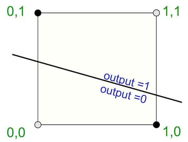
Canonical example: XOR function

• The positive/negative examples are not linearly separable.
• Need to map the input ($x_1,x_2$) to a feature space where examples are linearly separable.

(Figure from Raquel Urtasun & Rich Zemel)

Possible choice: $\phi(x_1, x_2) = \cos(\pi(x_1+x_2))$

so that $\phi(0,0)=\phi(1,1)=1$ and $\phi(0,1)=\phi(1,0)=-1$

One more example from Aeroacoustics

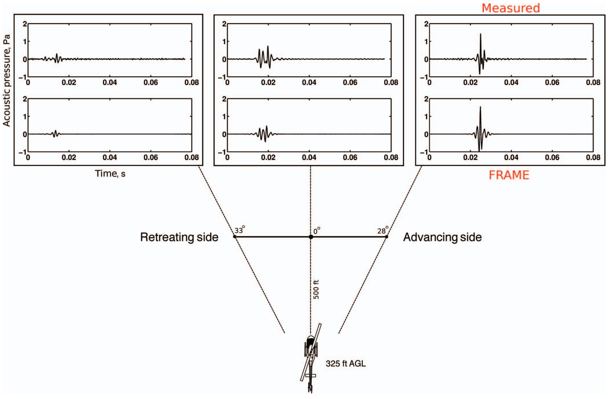(E. Greenwood, et al. JAHS 60, 022007 (2015))

One more example from Aeroacoustics

(E. Greenwood, et al. JAHS 60, 022007 (2015))

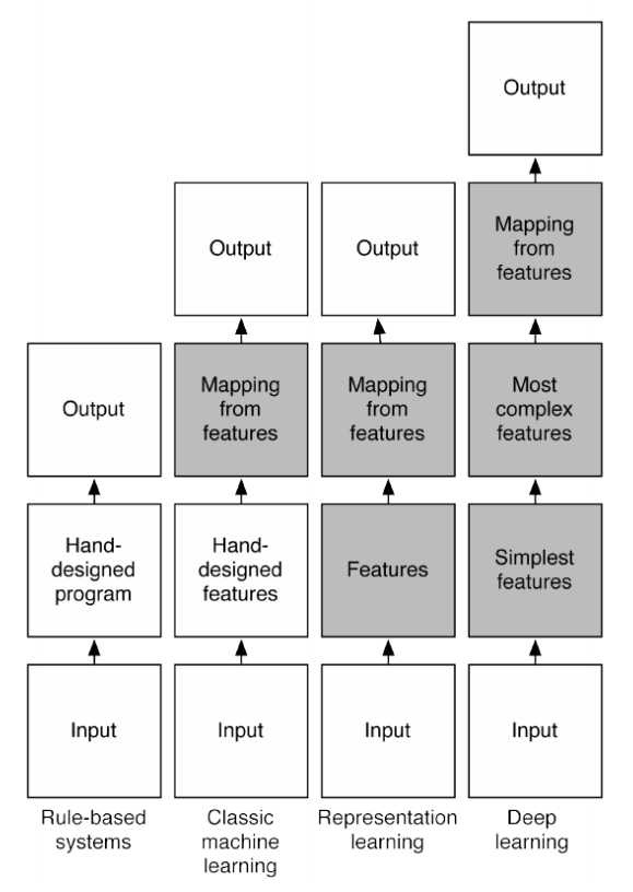
Drawbacks of handcrafting features

• Requires expert knowledge
• Requires time-consuming hand-tuning

This is why people are interested in neural networks, which can somehow figure out features from raw data.

Now recall this figure

Overview of Neural Networks

• Input Layer: provides input
• Hidden Layers: features extracted from input - there can be many
• Output Layer: output of the network
• Parameters (or weights) for each layer, $\theta^{(i)}$

Overview of Neural Networks

• A loss function is defined over the output units and desired outputs (i.e., labels) $$ \mathcal{L}\left( \textbf{y}, \hat{\textbf{y}}; \theta \right) \mbox{ where } \hat{\textbf{y}}=f(\textbf{x};\theta) $$
• The parameter of the network is trained to minimize the loss function based on gradient descent methods $$ \min_{\theta} \left[ \mathcal{L}\left( \textbf{y}, \hat{\textbf{y}}; \theta \right) \right] $$
• Forward Propagation (inference): Compute $\hat{\textbf{y}}=f(\textbf{x};\theta)$ (output given input)
• Backward Propagation (learning): Compute $\nabla_{\theta}\mathcal{L}$ (gradient of loss w.r.t. parameters)

Focus of Today: Forward Propagation

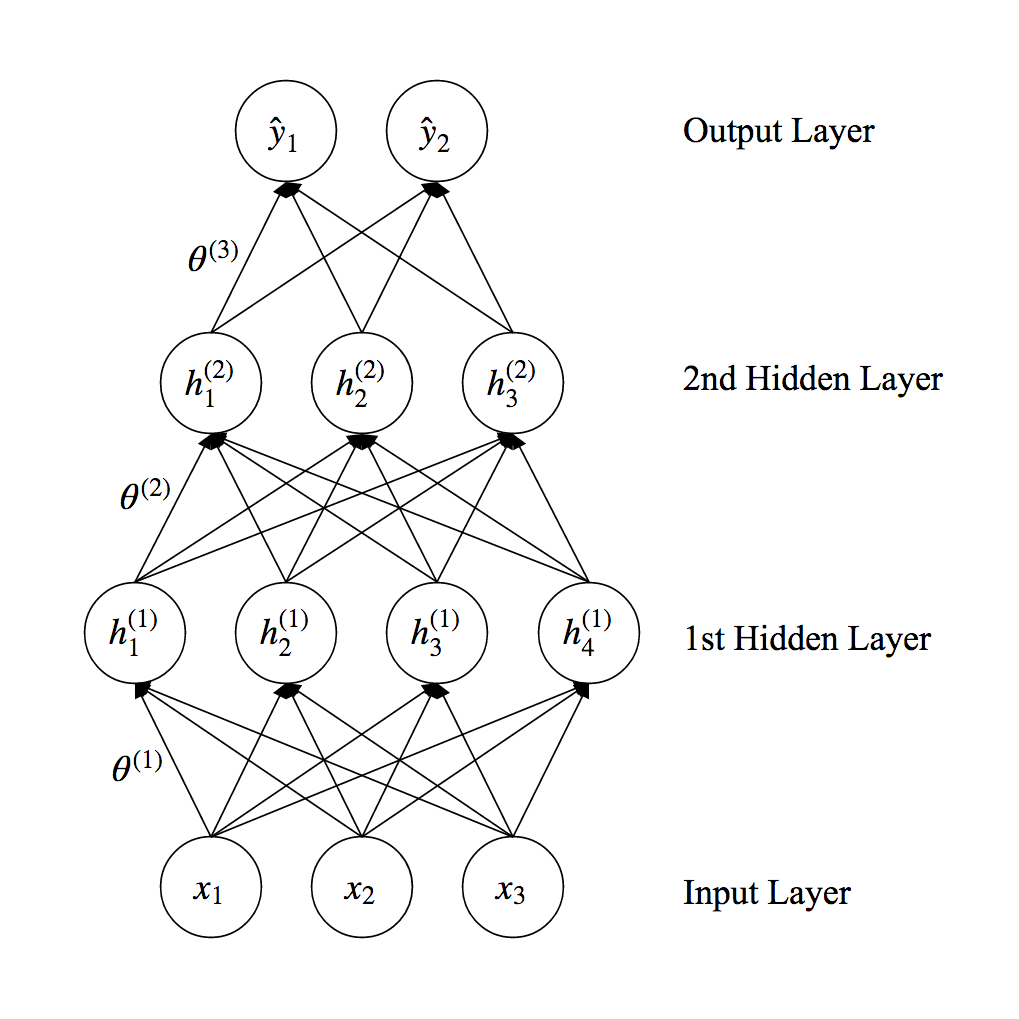
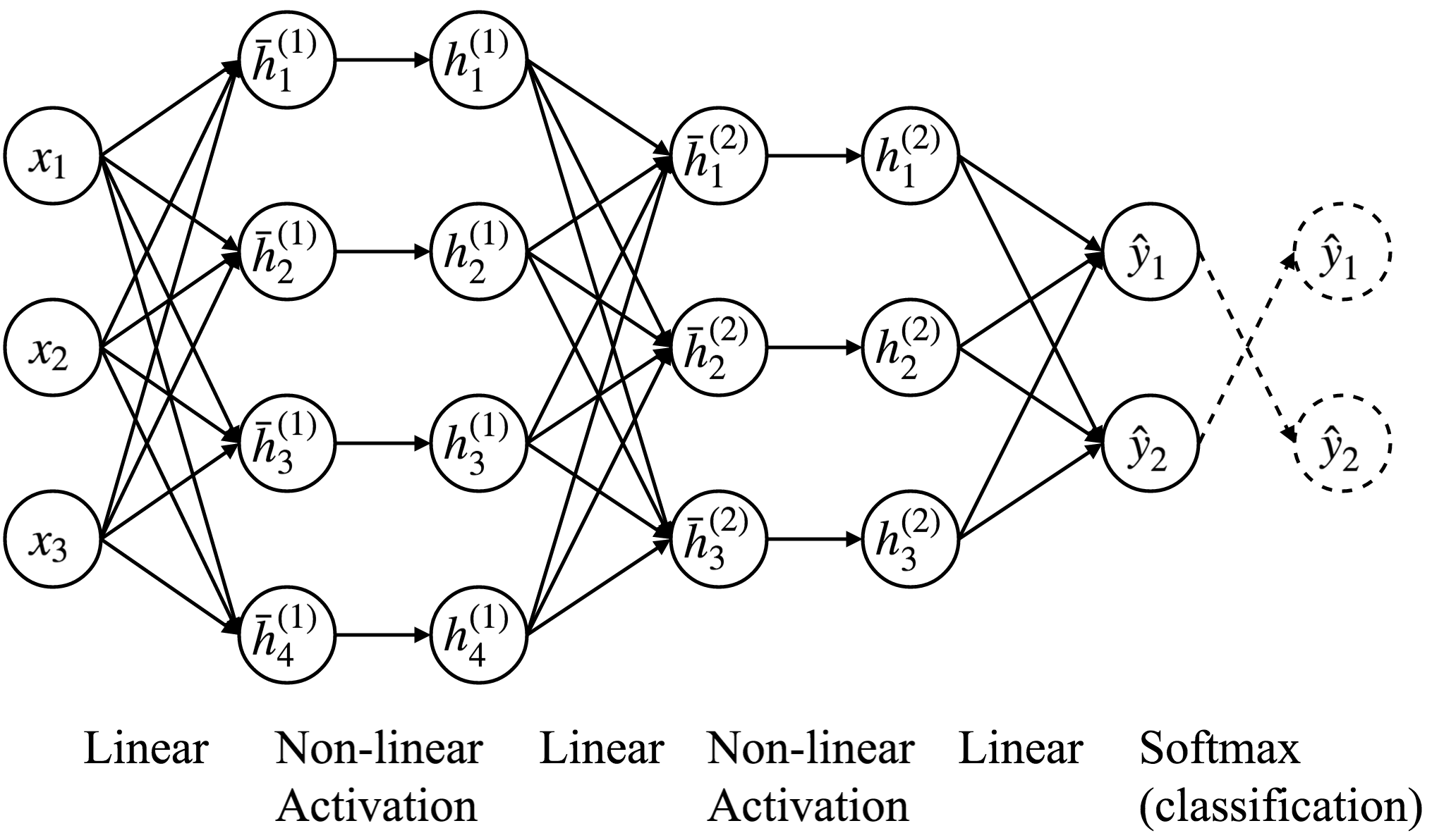
Forward Propagation

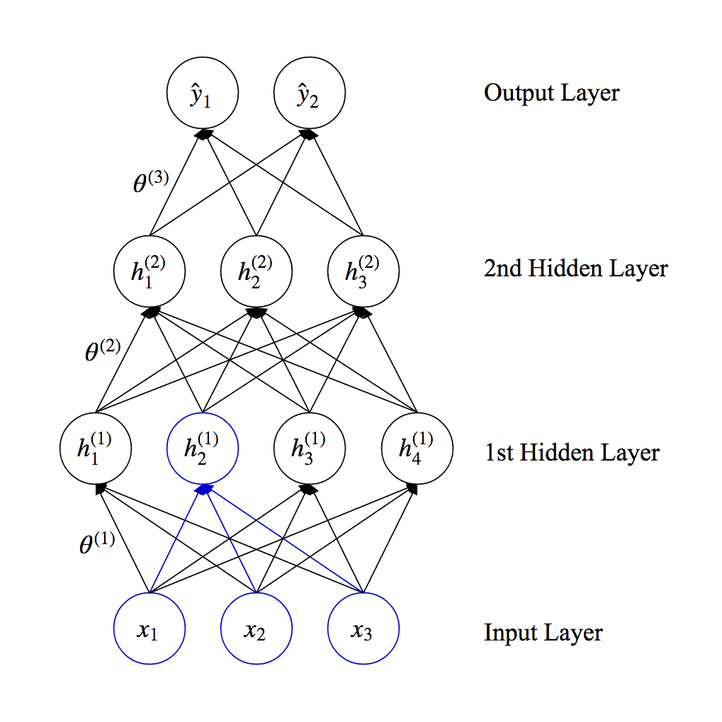
Forward Propagation

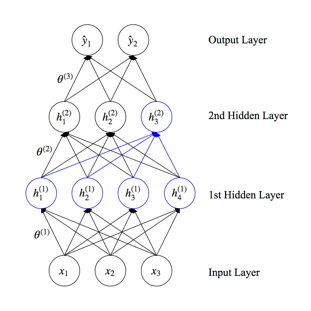
Forward Propagation

• The activation of each unit is computed based on the previous layer and parameters (or weights) associated with edges $$\underbrace{\textbf{h}^{(l)}}_{l\mbox{-th layer}}=f^{(l)}(\underbrace{\textbf{h}^{(l-1)}}_{(l-1)\mbox{-th layer}}; \underbrace{\theta^{(l)}}_{\mbox{weights}}) \mbox { where } \textbf{h}^{(0)} \equiv \textbf{x}, \textbf{h}^{(L)} \equiv \hat{\textbf{y}}$$ $$\hat{\textbf{y}}=f(\textbf{x};\theta)=f^{(L)} \circ f^{(L-1)} \cdots f^{(2)} \circ f^{(1)}\left(\textbf{x} ; \theta^{(1)} \right) $$

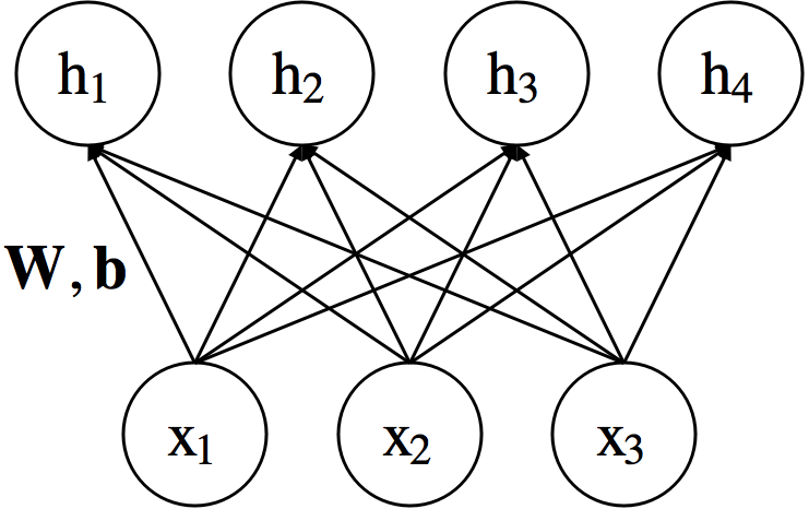
Types of Layers: Linear

$$ h_i=\sum_{j}w_{ij}x_j + b_i$$$$ \textbf{h} = \textbf{W}\textbf{x} + \textbf{b} $$

• $\textbf{x} \in \mathbb{R}^m $ : Input, $\textbf{h} \in \mathbb{R}^n $ : Output
• $\textbf{W} \in \mathbb{R}^{n \times m}$ : Weight, $\textbf{b} \in \mathbb{R}^{n}$ : Bias $\rightarrow$ parameter
• Often called "fully-connected layer"

Types of Layers: Non-linear Activation Function

• Applies a non-linear function to individual units.
• There is no weight.
• Allows neural networks to learn non-linear features.
• ex) Sigmoid, Hyperbolic Tangent, Rectified Linear Function

Non-linear Activation: Sigmoid

$$ h_i=\sigma (x_i) = \frac{1}{1+\exp\left(-x_i\right)} $$$$ \textbf{h} = \sigma \left(\textbf{x} \right) $$

xx = np.linspace(-5, 5, 100)
_=plt.plot(xx, 1/(1 + np.exp(-1 * xx)), '-g')

Non-linear Activation: Hyperbolic Tangent (Tanh)

$$ h_i= \mbox{tanh}(x_i)=\frac{\exp(x_i)-\exp(-x_i)}{\exp(x_i)+\exp(-x_i)} $$$$ \textbf{h} = \mbox{tanh} \left(\textbf{x} \right) $$

xx = np.linspace(-5, 5, 100)
_=plt.plot(xx, (np.exp(xx) - np.exp(-1 * xx))/(np.exp(xx) + np.exp(-1 * xx)), '-g')

Non-linear Activation: Rectified Linear (ReLU)

$$ h_i= \mbox{ReLU}(x_i)=\max\left(x_i, 0 \right) $$$$ \textbf{h} = \mbox{ReLU} \left(\textbf{x} \right) $$

Easier to optimize

xx = np.linspace(-5, 5, 101)
_=plt.plot(xx, xx * (xx > 0).astype(np.int), '-g')

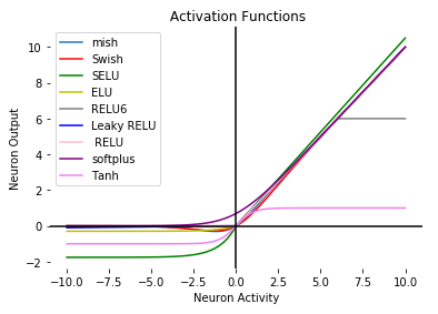
The ReLU family

• Smoother for gradient computation at $x=0$
• Adding contribution from the negative end
• Balance for computational cost

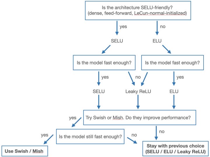
Flow chart for selecting ReLU-type activations

There are certainly more activation functions...

For example

• $\exp(-x^2)$ makes the NN similar to GPR's, and belongs to the "Radial Basis Function NN" (RBFNN)
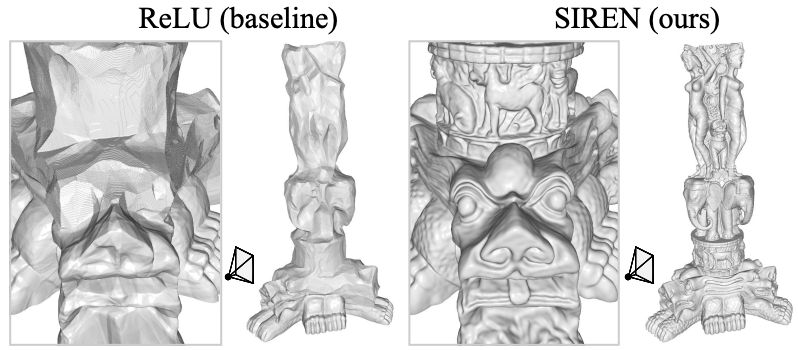
• $\sin(x)$ can work amazingly well in the reconstruction of complex signals (and their derivatives) [1]; example below

[1] Sitzmann, Vincent, et al. Implicit neural representations with periodic activation functions. Arxiv 2006.09661

Types of Layers: Softmax

$$ h_i = \frac{\exp(x_i)}{\sum_{j}\exp(x_j)} $$$$ \textbf{h} = \mbox{Softmax}(\textbf{x}) $$

• Note: $h_i \geq 0$ and $\sum_{i}h_i=1$
• Useful for generating a multinomial distribution (classification)

Multi-layer Neural Network

• Consists of multiple (linear + non-linear activation) layers.
• Each layer learns non-linear features from its previous layer.
• Often called Multi-Layer Perceptron (MLP).

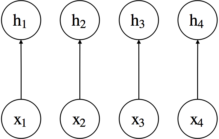
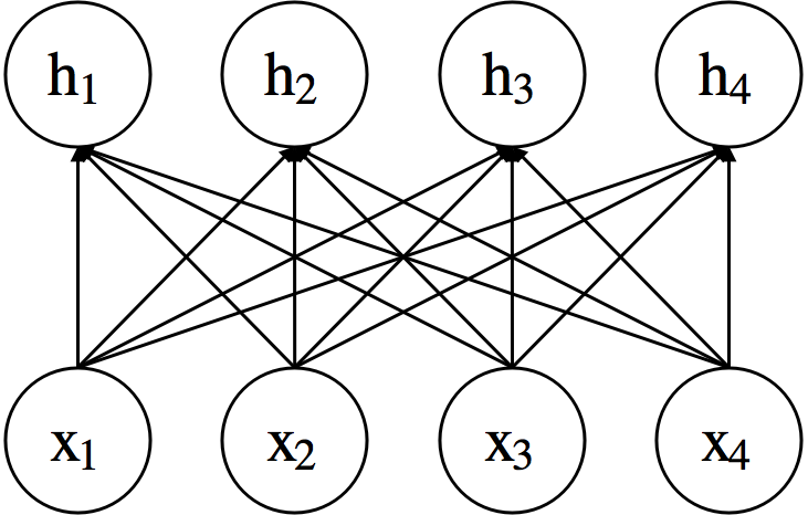
Multi-layer Neural Network

• Simplified illustration that only shows edges with weights.
• We assume that each layer is followed by a non-linear activation function (except for the output layer).

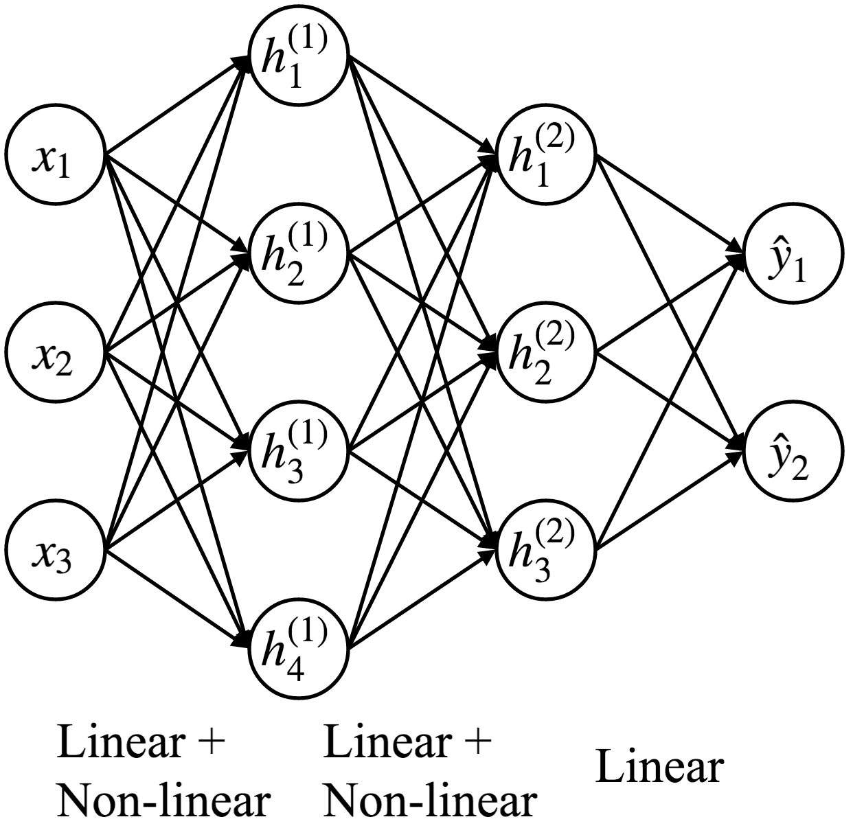
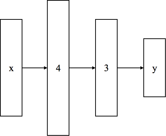
Multi-layer Neural Network

• More simplified illustration

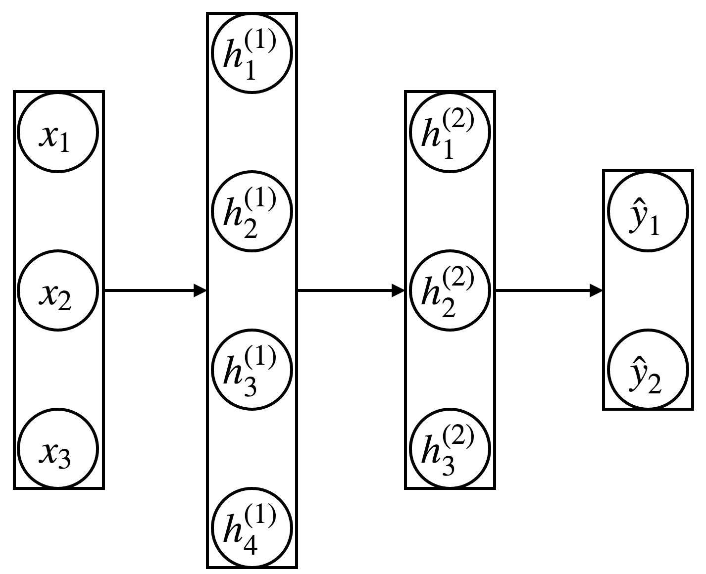
Multi-layer Neural Network

• Even more simplified illustration

MLP as universal functional approximation

2-layer MLP with infinite number of hidden units can approximate any functions.

• Classical result for shallow NN: to approximate a $C^n$-function (i.e. continuous up to $n$-th order derivative) on a $d$-dimensional set with infinitesimal error $\epsilon$ one needs a network of size about $O(\epsilon^{-d/n})$, assuming a smooth activation function [1]

[1] A. Pinkus, Approximation theory of the MLP model in neural networks, Acta numerica, 8(1999), 143-195.

• Deep NN - still under active research
  • For ReLU-based NN, it is equivalent to the finite element method
  • The $d$-dimensional $C^1$ functions can be represented with at most $\log_2(d + 1)$ hidden layers with size $O(\epsilon^{-d})$ (i.e. $n=1$). [2]
  • If the NN depth does not depend on $\epsilon$, the size $O(\mathrm{poly}(1/\epsilon))$; if the NN depth is $O(1/\epsilon)$, the size $(\mathrm{polylog}(1/\epsilon))$. [3]

[2] ReLU deep neural networks and linear finite elements arXiv:1807.03973

[3] Why Deep Neural Networks for Function Approximation? arXiv:1610.04161

Manual example: Piecewise linear curve fitting

Another (easier) exercise would be using sigmoid activation functions to do the XOR problem.

plt.plot(xx, yy, 'rs-', label='Target Function')
_=plt.legend()

• Linear+ReLU:

$h(x;k,b) = ReLU(kx+b)$

• Divide and conquer

plt.plot(xx, yy, 'rs-', label='Target Function')
plt.plot(xx, y2, 'bo-', label='Layer 1')
plt.plot(xx, yy-y2, 'g^--', label='Residual')
_=plt.legend()