Motivation
All models are wrong, but some are useful.
- In traditional CAE analysis, the physics cannot be precisely captured
- e.g. turbulence closure, constitutive relation modeling
- Uncertainty in prediction/design $\rightarrow$ Large safety factor and performance penalty
- In control and system engineering,
- Non-trivial to design a "clever" and robust controller for the complex and stochastic environment
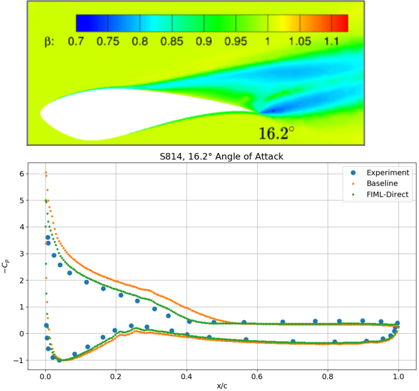
A machine learning model can be mebedded into the traditional analysis framework, so as to enhance the predictive capability of the latter.
 (Figure from Holland, Baeder etc. 2019)
Formulation
Notations
- $\cR(\vu)=0$ represents the governing equation of the problem, and the $\vu$ is state variable. For example,
- Fluid dynamics: $\cR$ - Navier-Stokes equation, $\vu$ - density, momentum, energy
- Solid mechanics: $\cR$ - Force equilibrium, $\vu$ - structural displacement
- System dynamics: $\cR$ - Rigid body motion, $\vu$ - linear & angular displacement/velocity
- $\cJ(\vu)$ is the model error, i.e. the difference between the theoretical model and the reality. For example,
- Fluid dynamics: Surface pressure of an airfoil is extracted from the fluid solution $\vu$ and compared to experimental measurement. The difference can be used as $\cJ$.
- Solid mechanics: Beam deformation - simulation vs. experiment.
- System dynamics: Dynamical response - simulation vs. experiment.
Calibration model
- $\vf=\cM(\vu;\vd)$ represents a machine learning model that is parameterized by $\vf$ and takes in the state variable $\vu$. It returns a set of coefficients $\vd$ to calibrate/correct the model prediction. For example,
- Fluid dynamics: $\vf$ to correct turbulence production term in the RANS equation, so as to improve the pressure prediction.
- Solid mechanics: $\vf$ to correct stress-strain relation, so as to improve the structural deformation prediction.
- System dynamics: $\vf$ to be used as an unknown external forcing term, so as to improve the accuracy of simulation.
- When $\cM$ is incorporated into the analysis framework, the governing equation becomes, $$ \cR(\vu;\vf)=0,\quad \mbox{where } \vf=\cM(\vu;\vd) $$ and similarly, the model error becomes $\cJ(\vu;\vf)$.
Optimization formulation
To improve the model, one wants to find the output of the calibration model that minimizes the model error, i.e. $$ \begin{align} \min_{\vf} &\quad \cJ(\vu;\vf) \\ \mathrm{s.t.} &\quad \cR(\vu;\vf) = 0 \end{align} $$
Two strategies to solve the optimization problem,
- Indirect approach:
- First, solve the optimization problem and find the optimal correction factors $\vf$.
- Then, using $\vf$ as training data, fit a calibration model $\vf=\cM(\vu;\vd)$.
- Pros: $\cM$ does not explicitly exist in the governing equation, so easy to implement
- Cons: Size of $\vf$ can be large, so inefficient to train; and accuracy may be sacrificed in model fitting.
- Direct approach:
- Implement the model $\cM$ in $\cR$ and $\cJ$ directly
- Solve a coupled optimization problem that generates the optimal parameters $\vd$ in the calibration model.
The direct approach is solving a slightly different optimization problem, $$ \begin{align} \min_{\vd} &\quad \cJ(\vu;\vd) \\ \mathrm{s.t.} &\quad \cR(\vu;\vd) = 0 \end{align} $$ where $\cJ$ is used the loss function to train the calibration model; the difficulty is the backpropagation through the equality constraint.
Adjoint Method for PDE Constraint
Consider the optimization problem in general, $$ \begin{align} \min_{\vtt} &\quad \cJ(\vu;\vtt) \\ \mathrm{s.t.} &\quad \cR(\vu;\vtt) = 0 \end{align} $$ where $\cR(\vu;\vtt) = 0$ is a set of $N$ equations representing the numerical discretization of a PDE. The size of $\vu$ can be way larger than the size of the design variables $\vtt$.
Given the design variables $\vtt^*$, the PDE is usually solved by a certain form of the Newton-Raphson method, $$ \begin{align} \ppf{\cR}{\vu}\Delta\vu^i &= -\cR(\vu^i,\vtt^*) \\ \vu^{i+1} &= \vu^i + \Delta\vu^i \end{align} $$ where the first equation is typically solved using an iterative method.
Formulation by adjoint variables
For optimization, one wants the full derivative of $\cJ(\vu;\vtt)$ w.r.t. $\vtt$, i.e. $$ \ddf{\cJ(\vu;\vtt)}{\vtt} = \ppf{\cJ}{\vu}\ppf{\vu}{\vtt} + \ppf{\cJ}{\vtt} $$ where $\ppf{\vu}{\vtt}$ is non-trivial to compute.
From the constraint, one knows, $$ \ddf{\cR(\vu;\vtt)}{\vtt} = \ppf{\cR}{\vu}\ppf{\vu}{\vtt} + \ppf{\cR}{\vtt} = 0 $$ or $$ \ppf{\vu}{\vtt} = \left(-\ppf{\cR}{\vu}\right)^{-1}\ppf{\cR}{\vtt} $$
Therefore, $$ \ddf{\cJ(\vu;\vtt)}{\vtt} = \ppf{\cJ}{\vu}\left(-\ppf{\cR}{\vu}\right)^{-1}\ppf{\cR}{\vtt} + \ppf{\cJ}{\vtt} $$
Now let $$ \vtf^T = -\ppf{\cJ}{\vu}\left(\ppf{\cR}{\vu}\right)^{-1} $$ or $$ \left(\ppf{\cR}{\vu}\right)^T\vtf = -\left(\ppf{\cJ}{\vu}\right)^T $$
This last equation is called the Adjoint Equation, and $\vtf$ is called the Adjoint Variable.
As a result, the full derivate of $\cJ(\vu;\vtt)$ w.r.t. $\vtt$ is computed as follows,
- Given $\vtt$, solve $\cR(\vu;\vtt)=0$ to find $\vu$
- In this process one obtains $\ppf{\cR}{\vu}$.
- Given $\vtt$ and $\vu$, find $\ppf{\cJ}{\vu}$, $\ppf{\cJ}{\vtt}$, and $\ppf{\cR}{\vtt}$.
- Solve the adjoint equation and find $\vtf$. $$ \left(\ppf{\cR}{\vu}\right)^T\vtf = -\left(\ppf{\cJ}{\vu}\right)^T $$
- The gradient of $\cJ$ $$ \ddf{\cJ(\vu;\vtt)}{\vtt} = \vtf^T\ppf{\cR}{\vtt} + \ppf{\cJ}{\vtt} $$
Formulation by Lagrange multipliers
Introduce a vector of Lagrange multipliers $\vtf$ $$ \cL(\vu;\vtt) = \cJ(\vu;\vtt) + \vtf^T \cR(\vu;\vtt) $$
Now one wants the full derivative of $\cL(\vu;\vtt)$ w.r.t. $\vtt$, i.e. $$ \ddf{\cL(\vu;\vtt)}{\vtt} = \ppf{\cJ}{\vu}\ppf{\vu}{\vtt} + \ppf{\cJ}{\vtt} + \vtf^T\left( \ppf{\cR}{\vu}\ppf{\vu}{\vtt} + \ppf{\cR}{\vtt} \right) $$
The RHS is $$ \ppf{\cJ}{\vtt} + \vtf^T\ppf{\cR}{\vtt} + \left(\ppf{\cJ}{\vu} + \vtf^T\ppf{\cR}{\vu}\right)\ppf{\vu}{\vtt} $$
One can eliminate $\ppf{\vu}{\vtt}$ by setting the bracket to zero, $$ \ppf{\cJ}{\vu} + \vtf^T\ppf{\cR}{\vu} = 0 $$ or the adjoint equation $$ \left(\ppf{\cR}{\vu}\right)^T\vtf = -\left(\ppf{\cJ}{\vu}\right)^T $$
Extra: Multiple PDE constraints
When a multi-physics problem is considered, which is not uncommon in the field of engineering, the optimization problem becomes $$ \begin{align} \min_{\vtt} &\quad \cJ(\vU;\vtt) \\ \mathrm{s.t.} &\quad \cR_j(\vU;\vtt) = 0,\quad j=1,\cdots,m \end{align} $$ where $m$ PDE's are involved, with unknowns $\vU=\{\vu_1,\cdots,\vu_m\}$.
Introduce a set of Lagrange multipliers, or the adjoint variables, $$ \cL(\vU;\vtt) = \cJ(\vU;\vtt) + \sum_{j=1}^m \vtf_j^T \cR_j(\vU;\vtt) $$
Take the full derivative, $$ \begin{align} \ddf{\cL(\vu;\vtt)}{\vtt} &= \ppf{\cJ}{\vU}\ppf{\vU}{\vtt} + \ppf{\cJ}{\vtt} + \sum_{j=1}^m \vtf_j^T\left( \ppf{\cR_j}{\vU}\ppf{\vU}{\vtt} + \ppf{\cR_j}{\vtt} \right) \\ &= \ppf{\cJ}{\vtt} + \sum_{j=1}^m \vtf_j^T\ppf{\cR_j}{\vtt} + \sum_{j=1}^m \left(\vtf_j^T\ppf{\cR_j}{\vU} + \ppf{\cJ}{\vU}\right)\ppf{\vU}{\vtt} \end{align} $$
A set of $m$ coupled adjoint equations is identified as $$ \sum_{j=1}^m \left(\ppf{\cR_j}{\vu_i}\right)^T\vtf_j = \left(\ppf{\cJ}{\vu_i}\right)^T,\quad i=1,\cdots,m $$
Back to Model Calibration
- The adjoint method can be readily applied to the indirect approach by letting $\vtt=\vf$.
- Slightly more involved for the direct approach, where $\vtt=\vd$:
$$
\ppf{\cR}{\vtt} = \ppf{\cR}{\vf}\ppf{\vf}{\vd}
$$
- $\ppf{\cR}{\vf}$: Same term in indirect approach.
- $\ppf{\vf}{\vd}$: A new term found by backpropagation of $\cM$
Numerical Example
We solve a 1D advection-diffusion equation for $x\in [0,1]$ $$ p u' - u'' = f(x;\vtt),\quad u(0)=u_0,\ u'(1)=n_1 $$ where $p$ is a constant, representing wave speed.
The RHS contains some unknown parameters $$ f(x;\vtt) = x^2 + \theta_1 x + \theta_2 $$
Suppose we know a solution $u^*$ found at the true parameters $\theta^*$. To infer $\theta^*$ from $u^*$, we solve $$ \begin{align*} \min_{\vtt} &\quad J(u;\vtt) \equiv \int_0^1 (u-u^*)^2 dx \\ \mathrm{s.t.} &\quad p u' - u'' = f(x;\vtt),\quad u(0)=u_0,\ u'(1)=n_1 \end{align*} $$
xx = np.linspace(0,1,41)
f = plt.figure(figsize=(6,4))
plt.plot(xx, fu(xx));
System Discretization
We use a generic Galerkin method to discretize the differential equation and the objective.
Specifically, we pick $N$ Legendre polynomials as basis functions, and represent the solution as $$ u(x) = \sum_{i=1}^N u_i\psi_i(x) \equiv \vty^T(x) \vu $$
f, ax = plt.subplots(ncols=2, figsize=(8,4))
for _i in range(0,5):
    ax[0].plot(xx, eval_leg0(_i, xx), label=f"Order={_i}")
    ax[1].plot(xx, eval_leg1(_i, xx))
ax[0].legend()
ax[0].set_title("Legendre polynomials")
ax[1].set_title("Derivatives");
The objective is converted to a quadratic form, $$ \cJ(\vu;\vtt) = \int_0^1 \left( \vty^T\vu - u^* \right)^2 dx \equiv \vu^T \vM \vu - 2\vu^T \vm + \text{const} $$ where $$ \vM = \int_0^1 \vty\vty^T dx,\quad \vm = \int_0^1 \vty u^* dx $$
The equation is converted to a linear system,
$$
\cR(\vu;\vtt) = \vA\vu - \vb(\vtt) = 0
$$
where for the formulation of $\vA$ see the Differential Equations slides in Math review, and
$$
\vb(\vtt) = \int_0^1 \vty f(x,\vtt) dx
$$
Adjoint-based Optimization
This brings us to the standard form: $$ \begin{align*} \min_{\vtt} &\quad \cJ(\vu;\vtt) \\ \mathrm{s.t.} &\quad \cR(\vu;\vtt) = 0 \end{align*} $$ Now suppose we start with an initial guess, say $\vtt^{(0)}=[10.0, 10.0]$.
Then, to use the adjoint formulation to obtain the gradients for optimization $\ddf{\cL(\vu;\vtt)}{\vtt}$ at $\vtt^{(0)}$ -
First, we solve $\vu^{(0)}$ at $\vtt^{(0)}$. Clearly this is totally off.
theta0 = [10.0, 10.0]
sol, mats = galerkin(M, N, p, ub, nb, theta0)
print(obj(sol)[0])
compare_sol(sol, fu, 41);
0.6717431265076287
Then, we solve the adjoint problem $$ \left(\ppf{\cR}{\vu}\right)^T\vtf = -\left(\ppf{\cJ}{\vu}\right)^T $$ where $\ppf{\cR}{\vu}=\vA$, $\ppf{\cJ}{\vu}=(2\vM\vu-2\vm)^T$
And evaluate the gradients $$ \ddf{\cL(\vu;\vtt)}{\vtt} = \ppf{\cJ}{\vtt} + \vtf^T \ppf{\cR}{\vtt} $$ where $\ppf{\cJ}{\vtt}=0$ and $\ppf{\cR}{\vtt}=-\ppf{\vb}{\vtt}$
Adjoint-based gradients, verified by finite difference:
# Adjoint
sol, mats = galerkin(M, N, p, ub, nb, theta0)  # Forward solve
_, gda = galerkin_da(sol, mats, obj)           # Adjoint/Backward solve
# Finite difference, using a SciPy function
def Jfd(qs):
    sol, _ = galerkin(M, N, p, ub, nb, qs)
    d, _ = obj(sol)
    return d
gfd = approx_fprime(theta0, Jfd)

print(f"Adjoint: {gda}, FD: {gfd}")
Adjoint: [0.04238442 0.09196361], FD: [0.04238444 0.09196366]
Now let's use a vanilla optimizer from SciPy to solve the problem (i.e., train the model)
def Jda(qs):
    sol, mats = galerkin(M, N, p, ub, nb, qs)
    fun, grd = galerkin_da(sol, mats, obj)
    return fun, grd
res = minimize(Jda, theta0, method="l-bfgs-b", jac=True)
print(res)
      fun: 7.840073109167548e-09
 hess_inv: <2x2 LbfgsInvHessProduct with dtype=float64>
      jac: array([-2.01714204e-08, -4.43224716e-08])
  message: 'CONVERGENCE: NORM_OF_PROJECTED_GRADIENT_<=_PGTOL'
     nfev: 8
      nit: 4
     njev: 8
   status: 0
  success: True
        x: array([ 0.00034045, -0.00022833])
# Check the converged solutions, i.e., "learned" model
sol, mats = galerkin(M, N, p, ub, nb, res.x)
compare_sol(sol, fu, 41);
# Note that much more cost would be incurred if we optimize
# by BRUTAL force (i.e., finite difference)
res = minimize(Jfd, theta0, method="l-bfgs-b", jac=False)
print(res)  # Look at `nfev`: function evaluation
      fun: 7.840448019872488e-09
 hess_inv: <2x2 LbfgsInvHessProduct with dtype=float64>
      jac: array([-3.35777998e-08, -7.81670232e-08])
  message: 'CONVERGENCE: NORM_OF_PROJECTED_GRADIENT_<=_PGTOL'
     nfev: 24
      nit: 4
     njev: 8
   status: 0
  success: True
        x: array([ 0.00038461, -0.00025382])
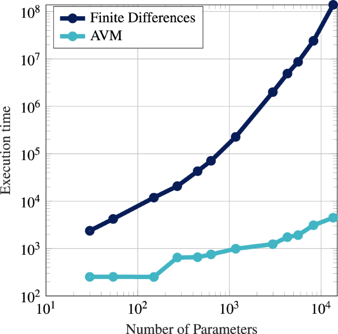
Key take-away: Adjoint formulation enables machine learning with large scale simulations.
 (Figure from Neustock et al. Nature 2019)