Machine Learning for Engineering

Neural Networks: Gradient Descent

Instructor: Daning Huang

TODAY: Neural Networks - II

• Loss functions
• Newton-type methods
• Gradient descent methods

References

• PRML Chp. 5
• Referenced papers

Training Neural Networks

Repeat until convergence

• $(\textbf{x},\textbf{y}) \leftarrow$ Sample an example (or a mini-batch) from data
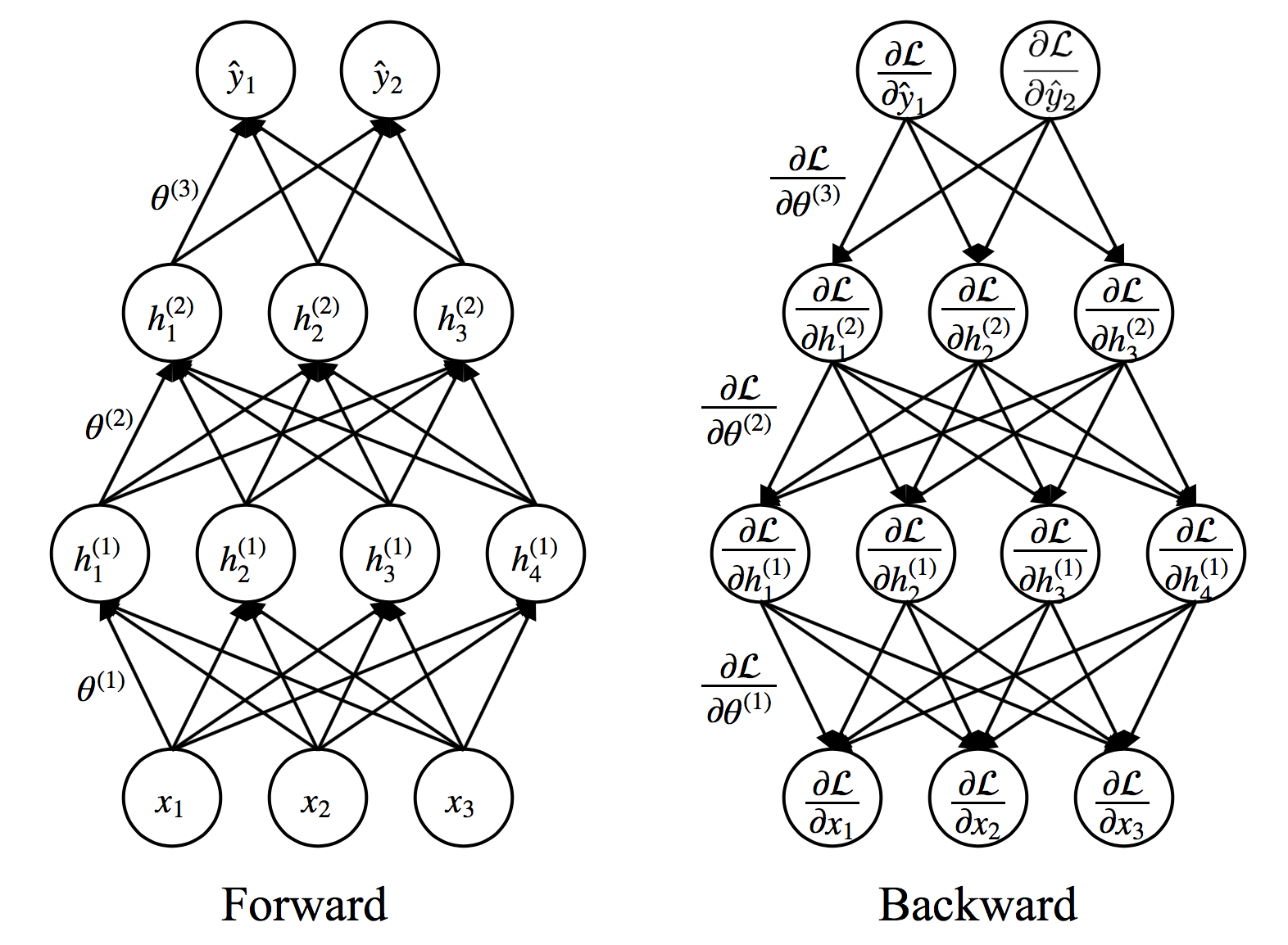
• $\hat{\textbf{y}} \leftarrow f\left( \textbf{x} ; \theta \right)$ Forward propagation
• Compute $\mathcal{L}\left(\textbf{y},\hat{\textbf{y}}\right)$
• $\nabla_{\theta}\mathcal{L} \leftarrow$ Backward propagation
• Update weights using (stochastic) gradient descent
  • $\theta \leftarrow \theta - \alpha \nabla_{\theta}\mathcal{L}$

Types of Losses: Squared Loss

$$ \mathcal{L}\left(\textbf{y},\hat{\textbf{y}}\right) = \frac{1}{2}\left\Vert \textbf{y}-\hat{\textbf{y}}\right\Vert^2_2 $$ $$ \frac{\partial\mathcal{L}}{\partial \hat{y}_i}=\hat{y}_i-y_i \iff \nabla_{\hat{\textbf{y}}}\mathcal{L}=\hat{\textbf{y}}-\textbf{y} $$

• Used for regression problems

Forward/Backward propagation

We are going to cover backward propagation in the next lecture.

Newton's Method: Overview

• Goal: Minimize a general function $F(w)$ in one dimension by solving for $$ f(w) = \frac{\partial F}{\partial w} = 0 $$
• Newton's Method: To find roots of $f$, Repeat until convergence: $$ w \leftarrow w - \frac{f(w)}{f'(w)} $$

Geometric Intuition

• Find the roots of $f(w)$ by following its tangent lines. The tangent line to $f$ at $w_{k-1}$ has equation $$ \ell(w) = f(w_{k-1}) + (w-w_{k-1}) f'(w_{k-1}) $$
• Set next iterate $w$ to be root of tangent line: $$ \begin{gather} f(w_{k-1}) + (w-w_{k-1}) f'(w_{k-1}) = 0 \\ \implies \boxed{ w = w_{k-1} - \frac{f(w_{k-1})}{f'(w_{k-1})} } \end{gather} $$

Application to minimization

To minimize $F(w)$, find roots of $F'(w)$ via Newton's Method.

Repeat until convergence: $$ \boxed{w \leftarrow w - \frac{F'(w)}{F''(w)}} $$

Minimization in multivariate case

Replace second derivative with the Hessian Matrix, $$ H_{ij}(w) = \frac{\partial^2 F}{\partial w_i \partial w_j} $$

Newton update becomes: $$ \boxed{ w \leftarrow w - H^{-1} \nabla_w F} $$

• Advantage: Fast convergence (quadratic)
• Disadvantage: Computing Hessian and its inverse is slow

Sometimes line search is necessary

Let $p=-H^{-1} \nabla_w F$, find a step size $\alpha$ such that $$ \min_\alpha F(w+\alpha p) $$ Then $$ \boxed{ w \leftarrow w - \alpha H^{-1} \nabla_w F} $$

Issues

• Computing Hessian is expensive
  • Approximate linear solve for $H^{-1}$
  • Quasi-Newton methods: Construct approximate $H$ from past gradients (e.g. BFGS using secant equation) $$\mbox{Scalar:}\quad F''(w_{k+1}) \approx [F'(w_{k+1}) - F'(w_k)]/(w_{k+1}-w_k)$$ $$\mbox{Vector:}\quad H_{k+1}(w_{k+1}-w_k) \approx \nabla_w F(w_{k+1}) - \nabla_w F(w_k)$$

• Do not work well for non-convex problems
  • It only solves for $\nabla_w F=0$
  • The solution can be a saddle point, or even a maximizer!
  • Possible to use the Levenberg-Marquardt algorithm (regularizing the Hessian) $$\tilde{H} = \lambda I + H,\quad \lambda>0$$

Unfortunately, saddle points prevail in high dimensions

The $\epsilon-\alpha$ curve [1]

• $\alpha$: Percentage of negative eigenvalues of Hessian at critical point (i.e. gradient=0)
• $\epsilon$: Error at critical point
• There are many saddle points (the figure is for a relatively small NN)
• Strong positive correlation between $\alpha$ and $\epsilon$, esp. in high-dim optimization

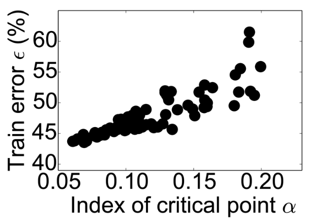
[1] Y. Dauphin et al. Identifying and attacking the saddle point problem in high-dimensional non-convex optimization. NeurIPS 2014.

Intuitively, in high dimensions, the chance that all the directions around a critical point lead upward (positive curvature) is exponentially small w.r.t. the number of dimensions

Implications:

• If you get a "converged" model and it does not perform well, then the model is likely at a saddle point
• The local minima are likely to be as good as global minima
  • For even larger problems, even saddle points with low index are sufficient (which is more common)
• Now that Hessian-based method might be problematic, we should just use Gradient Descent

Simple Gradient Descent

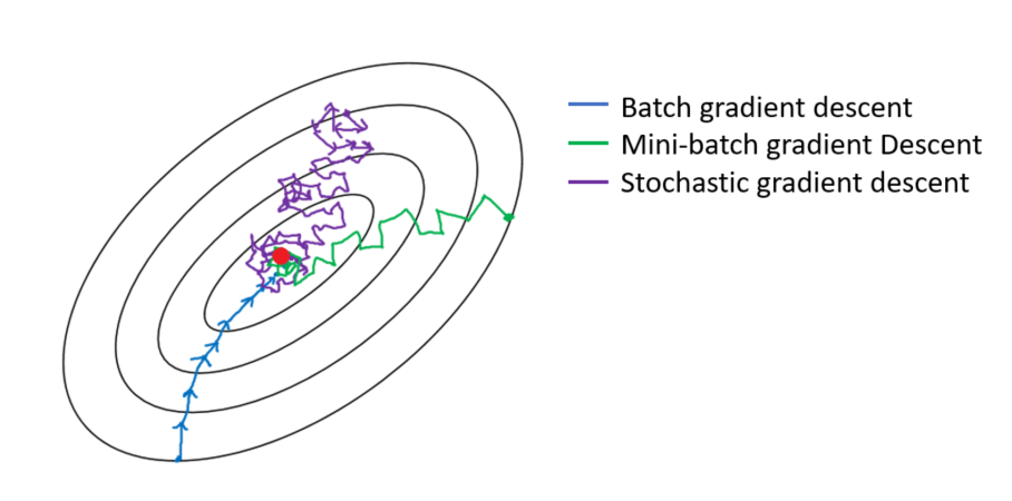
Batch mode

Given dataset $\{ (x,t) \}$ and initial guess $\theta_0$, repeat until convergence:

• $\theta = \theta - \eta \nabla_\theta \mathcal{L}(\theta)$

where $\eta$ is the step size(s), or learning rate, and assuming quadratic loss,

$$ \nabla_\theta \mathcal{L}(\theta) = \sum_{n=1}^N \left[ f\left( \textbf{x}^{(n)} ; \theta \right) - y^{(n)} \right] \frac{\partial f\left( \textbf{x}^{(n)} ; \theta \right)}{\partial \theta} $$

• Disadvantage: Can be slow if the network is large and the dataset is huge

Stochastic mode, a.k.a., Stochastic Gradient Descent (SGD)

Main Idea: Instead of computing batch gradient (over entire training data), just compute gradient for individual example and update.

Repeat until convergence: for $n=1,\dots,N$

$$ \theta = \theta - \eta \nabla_\theta \mathcal{L}(\textbf{x}^{(n)}; \theta) $$

where

$$ \nabla_\theta \mathcal{L}(\textbf{x}^{(n)}; \theta) = \left[ f\left( \textbf{x}^{(n)} ; \theta \right) - y^{(n)} \right] \frac{\partial f\left( \textbf{x}^{(n)} ; \theta \right)}{\partial \theta} $$

• Advantage: Easier to compute, esp. when the dataset is huge; sometimes can escape local minima
• Disadvantage: The gradient becomes noisy - impacts convergence; the Hessian is not well-defined even if we want to use it
• In between there are "mini-batch" mode

Comparison - Batch mode seems more reliable?

Comparison - but if we look at cost

• Think LBFGS as batch GD
• SGD shows fast initial progress, though slowed down later.

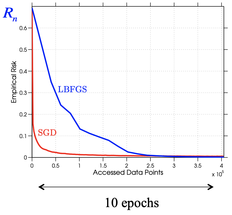
Let $n$ be the batch size, $\epsilon\sim 10^{-3}$ the final "loss", $T$ the allowable time, then [1]

• Batch: Work$\sim n\log(1/\epsilon)$, Error$\sim(\log(T)+1)/T$ - better to focus on a certain number of samples
• Stochastic: Work$\sim 1/\epsilon$, Error$\sim 1/T$ - just process as many samples as possible

[1] L. Bottou, et al. Stochastic Gradient Methods For Large-Scale Machine Learning. Arxiv: 1606.04838; Also here as slides: http://users.iems.northwestern.edu/~nocedal/ICML

Practical SGD methods

$$ \theta = \theta - \eta \nabla_\theta \mathcal{L}(\textbf{x}^{(n)}, \theta) $$

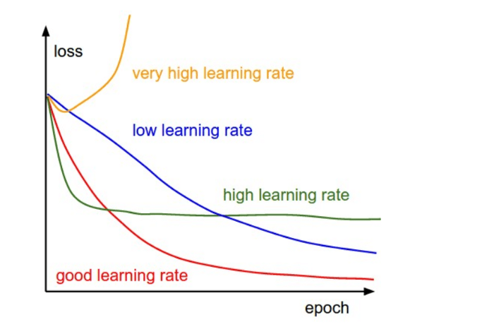
• How to determine learning rate?
• How to improve convergence rate?
• Getting out of saddle points?

Fancier variants

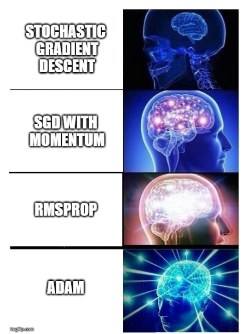
SGD with momentum

Let the optimizer remember the previous gradients, $$ v_k = \rho v_{k-1} + (1-\rho)\nabla_\theta F(\theta_k) $$ Then $$ \boxed{ \theta_{k+1} = \theta_k - \eta v_k} $$

• Momentum is a weighted sum of gradients, weights for old gradients decay exponentially
• Less sensitive to noise
• Easier to pass local minimum

AdaGrad

Let the optimizer tune learning rate automatically, $$ g_k = g_{k-1} + [\nabla_\theta F(\theta_k)]^2 $$ Then $$ \boxed{ \theta_{k+1} = \theta_k - \frac{\eta}{\sqrt{g_k}+\epsilon} \nabla_\theta F(\theta_k)} $$

• Note that the square and sqrt are element-wise, $\epsilon\sim 10^{-6}$ to avoid division by zero
• Learning rate decreases as the solution moves longer distance
• Now $\eta$ can be very large - It will become small anyways

RMSProp

Similar to AdaGrad, but allow the optimizer to "forget", $$ g_k = \alpha g_{k-1} + (1-\alpha)[\nabla_\theta F(\theta_k)]^2 $$ Then $$ \boxed{ \theta_{k+1} = \theta_k - \frac{\eta}{\sqrt{g_k}+\epsilon} \nabla_\theta F(\theta_k)} $$

• Like momentum, let old squared gradient decay exponentially. Typically $\alpha=0.9$.
• The rest is AdaGrad.

Adam

Combine the best of SGD w/ momentum and RMSProp, $$v_k = \beta_1 v_{k-1} + (1-\beta_1)\nabla_\theta F(\theta_k)$$ $$g_k = \beta_2 g_{k-1} + (1-\beta_2)[\nabla_\theta F(\theta_k)]^2$$ Then $$ \boxed{ \theta_{k+1} = \theta_k - \frac{\eta}{\sqrt{g_k}+\epsilon} v_k} $$

• Sometimes $v_k$ and $g_k$ are corrected before updating $\theta$, $$ v_k \leftarrow \frac{v_k}{1-\beta_1^k},\quad g_k \leftarrow \frac{g_k}{1-\beta_2^k} $$
• It was suggested to use $\beta_1=0.9$, $\beta_2=0.999$.

More methods

People have devised many, many other gradient-descent methods. Some perform the best in some specific applications, but there is not "one-for-all" solution.

You will implement one of them in HW3.

There are also attempts to combine the advantages of different methods, e.g. [1]

[1] N. Keskar, R. Socher, Improving Generalization Performance by Switching from Adam to SGD, Arxiv 1712.07628

Visual comparison of the methods - I

From https://ruder.io/optimizing-gradient-descent/:

Visual comparison of the methods - II

From ruder.io:

Again, Deep NN's are filled with saddle points

xs = [[-1.5,0.5], [0.5, 1.5], [1.0, -1.0]]
res = batch_gradDesc(FGH, xs, NR(0.0), ifLS=True)  # Non-zero parameter for Levenberg-Marquardt
f1, ax = pltFunc(); batch_pltRes(ax, res)

xs = [[-1.5,0.5], [0.5, 1.5], [1.0, -1.0]]
ss = 0.5  # Noise in gradient

# res = batch_gradDesc(FGHS(ss), xs, fixLR(0.00001))
# res = batch_gradDesc(FGHS(ss), xs, GDM(0.00001,0.9))
# res = batch_gradDesc(FGHS(ss), xs, AdaGrad(2.0))
# res = batch_gradDesc(FGHS(ss), xs, RMSProp(0.1,0.9))
res = batch_gradDesc(FGHS(ss), xs, Adam(0.1,0.9,0.999))
f1, ax = pltFunc(); batch_pltRes(ax, res)

One more awesome interactive visualization: https://github.com/lilipads/gradient_descent_viz

Now that we know there are many saddle points and local minima...

• What kind of local minima is better? The flat ones - (empirically) better generalization performance
• Compare Adam and vanilla SGD [1]
  • Adam escapes saddle point easier (see the GIF earlier)
  • SGD favors flat minima more

Additional conclusion from [1]: A small learning rate or large-batch makes it much harder to escape from sharp minima

[1] Z. Xie. A Diffusion Theory For Deep Learning Dynamics: Stochastic Gradient Descent Exponentially Favors Flat Minima. Arxiv: 2002.03495

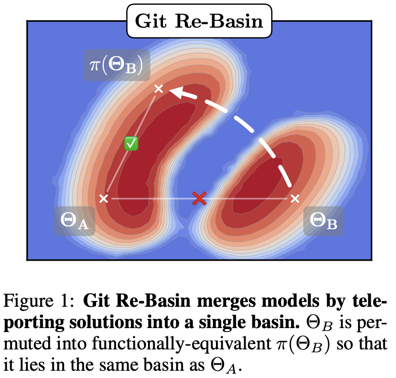
... And after all there are not that many local minima

Say we have trained a NN and then permute two neurons in a fully-connected layer

• The model parameters change from $\Theta_A$ to $\Theta_B$
• But the model output does not change and is "functionally equivalent"
• Even a simple MLP with 3 layers and 512 width has $10^{3498}$ equivalent permutations
  • Namely $(512!)^3$, ! for factorial

[1] S. Ainsworth et al. Git Re-Basin: Merging Models modulo Permutation Symmetries. ICLR 2023.

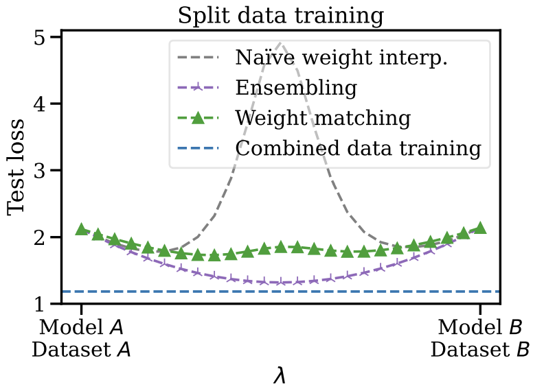
Linear mode connectivity

• One can permute $\Theta_B'=\pi(\Theta_B)$ so $\Theta_A$ and $\Theta_B'$ are in the same basin
• Varying parameters $\Theta(\lambda)=(1-\lambda)\Theta_A+\lambda\Theta_B$ experiences a bump in loss
• ... but $\Theta_A\rightarrow\Theta_B'$ does not!

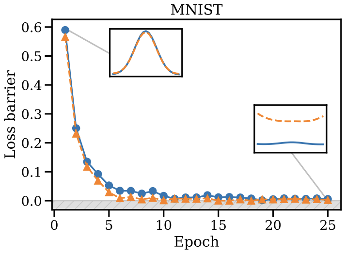
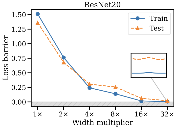
Further take-away

• Left: SGD favors one of the equivalent models during training
• Right: A wider model has more permutations and is easier for SGD to find better model

One possible intuition: SGD somewhat moves randomly; when there are many equivalent basins, it is more likely for it to hit one basin.

Practical aspects in training

• General procedure
• Techniques for improved convergence and better solutions

Basics: General procedure

• If there are not much data - try cross-validation to use all data
  • i.e., do splits of train-test, so that all data points are used as test once.
  • See Linear Regression module for review.
• Otherwise, do a split of train-valid-test.
  • Train: for decreasing the loss
  • Valid: for picking the best parameter during training (behave like test in CV)
  • Test: Completely unseen in the training process, used to verify the model performance

Basics: Diagnose your loss curve

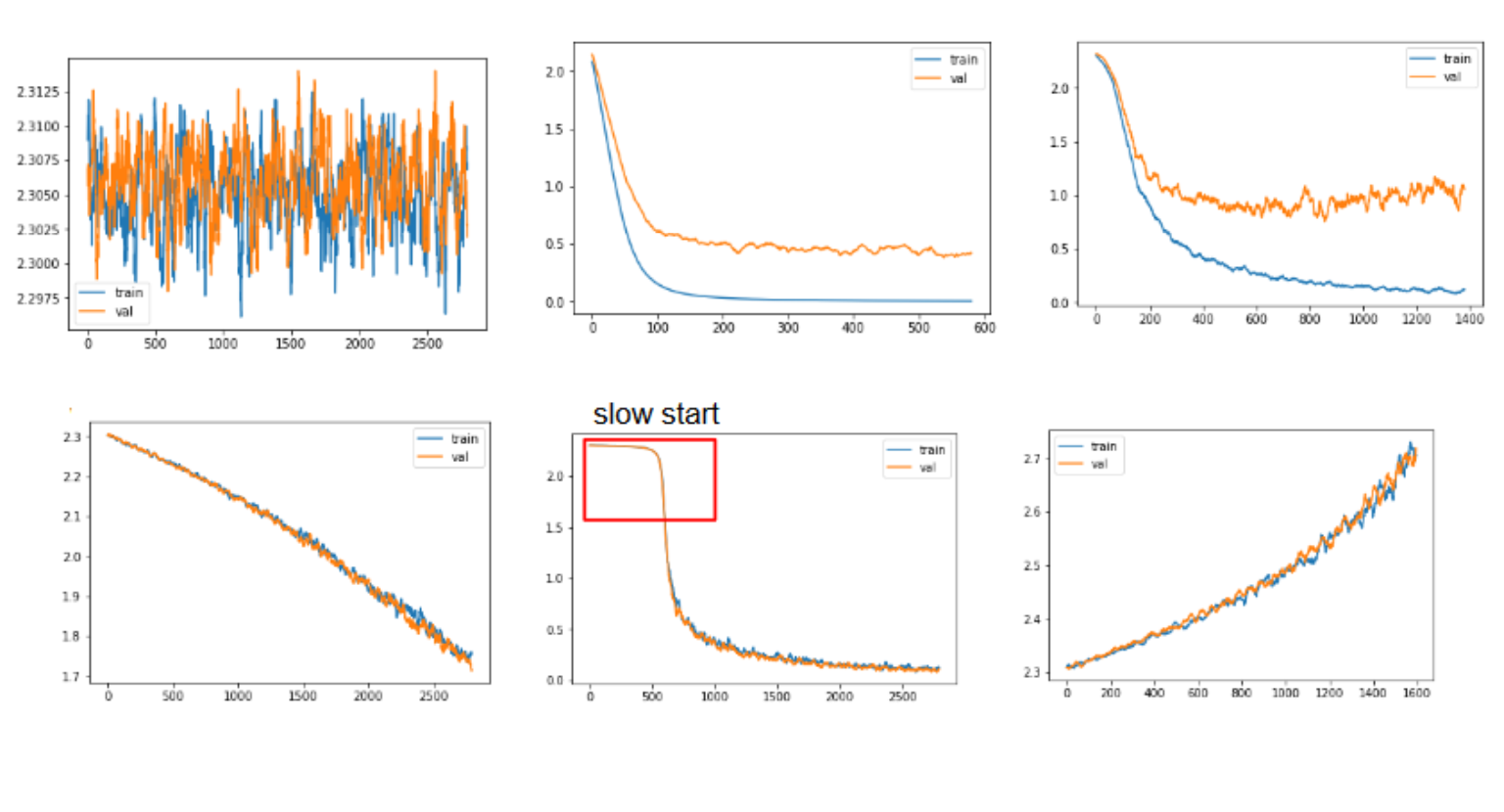
• Linearly decrease: increase the learning rate
• Shaky curves: increase the batch size
• Distant train/valid curves: overfitting
• Overlapping train/valid curves: underfitting

Basics: More on loss curves

dev=valid

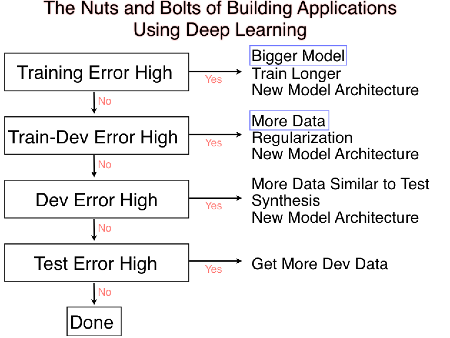
[1] A. Ng, Nuts and Bolts of Building Applications using Deep Learning, NeurIPS 2016

Intermediate: Caveats and Tuning tricks - I

• Always normalize and shuffle your data!

  • But normalization factors should be based on training dataset only.

• Pick the right learning rate: e.g., Grid search [1], or (cyclic) scheduling [2,3]

  • Higher learning rate for larger batch size (and larger batch-size if you have a bigger machine)

[1] S. Gugger, How Do You Find A Good Learning Rate

[2] I. Loshchilov, SGDR: Stochastic gradient descent with warm restarts, Arxiv: 1608.03983

[3] L. Smith, Cyclical Learning Rates for Training Neural Networks, 2017

Intermediate: Caveats and Tuning tricks - II

• Pick the right optimizer: Typically start with Adam, fine-tune with SGD

• Start with ReLU or tanh for activation; avoid sigmoid unless for "gate"-like layers

• Try overfitting on a small dataset

  • If your code/model is correct, the training should converge really fast

• Record your training experiments - learn from history

More techniques

[1] R. Sun. Optimization for deep learning: theory and algorithms. Arxiv 1912.08957 A nice comprehensive summary

More techniques - Weight initialization

• Basically to get better initial guesses of the weights [1,2]
• Let $n_i$ be input size, $n_o$ output size, so the weight $W$ of size $(n_i,n_o)$ and let $n=n_i$ or $n=(n_i+n_o)/2$
• Uniform $U[-s,s]$
  • Xavier (tanh/sigmoid): $s=\sqrt{3/n}$
  • Kaiming (ReLU): $s=\sqrt{6/n}$
• Gaussian $N(0,\sigma^2)$
  • Xavier (tanh/sigmoid): $\sigma=\sqrt{1/n}$
  • Kaiming (ReLU): $\sigma=\sqrt{2/n}$

[1] X. Glorot, et al. Understanding the difficulty of training deep feedforward neural networks. AISTATS 2010

[2] K. He, et al. Delving Deep into Rectifiers: Surpassing Human-Level Performance on ImageNet Classification. 1502.01852

More techniques - Dropout

• Randomly "throw away" neurons during training
  • so these neuron do not contribute to the prediction and their weights are not updated.
  • This is as if multiple NNs are being learned during training
• Avoids overfitting, since now there is a "committee" of NNs

[1] G. Hinton, et al. Improving neural networks by preventing co-adaptation of feature detectors. Arxiv:1207.0580

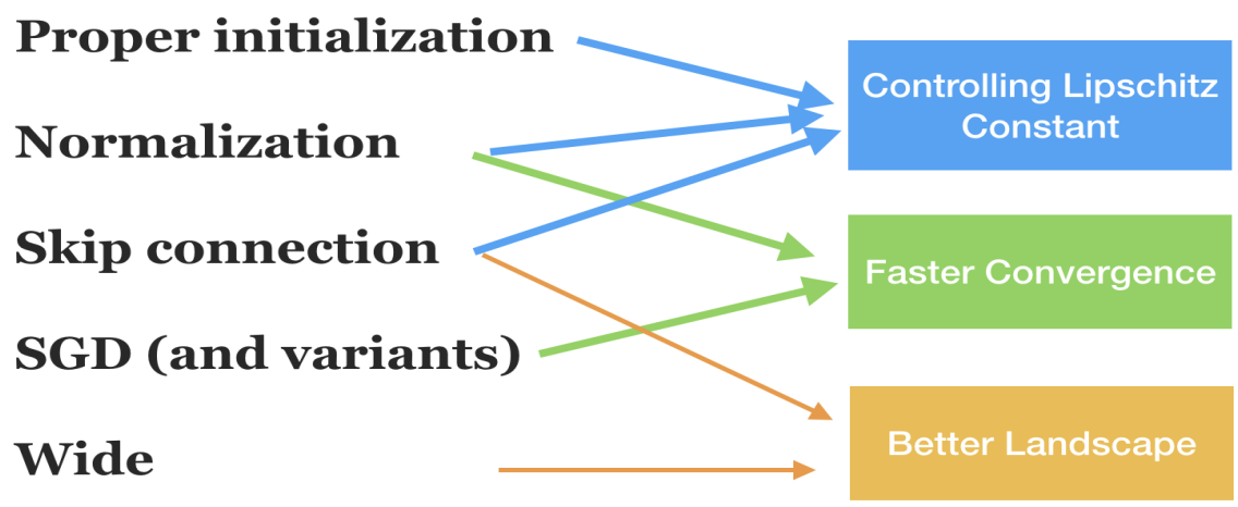
More techniques - Normalization within Network - I

• If we think each NN layer is a small model that we want to fit
  • Then it is natural to think about normalizing the "inputs" to these layers
  • The inputs, however, are the outputs of the preceeding layer

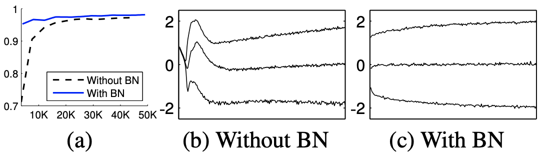
• Batch Normalization [1] does the trick
  • Turns out it maintains the distribution of inputs/outputs of the NN layers
  • Leads to faster convergence and perhaps better accuracy

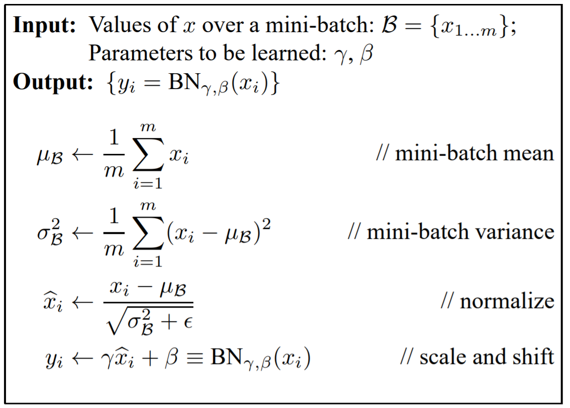
[1] S. Ioffe, et al. Batch normalization: Accelerating deep network training by reducing internal covariate shift. ICML 2015.

More techniques - Normalization within Network - II

• There are more variants, too, such as weight/layer/instance/group normalization etc.
  • See weight normalization [2] for example, it reparametrizes the weights instead of the inputs.

[2] T. Salimans, et al. Weight normalization: A simple reparameterization to accelerate training of deep neural networks. NeurIPS 2016

More techniques - Skip connection

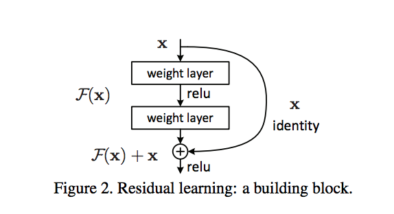
• This is an important type of NN architecture. It improves the convergence and has deeper implications.
• We will come back to this when talking about NN architectures.

Pursuing zero training error?

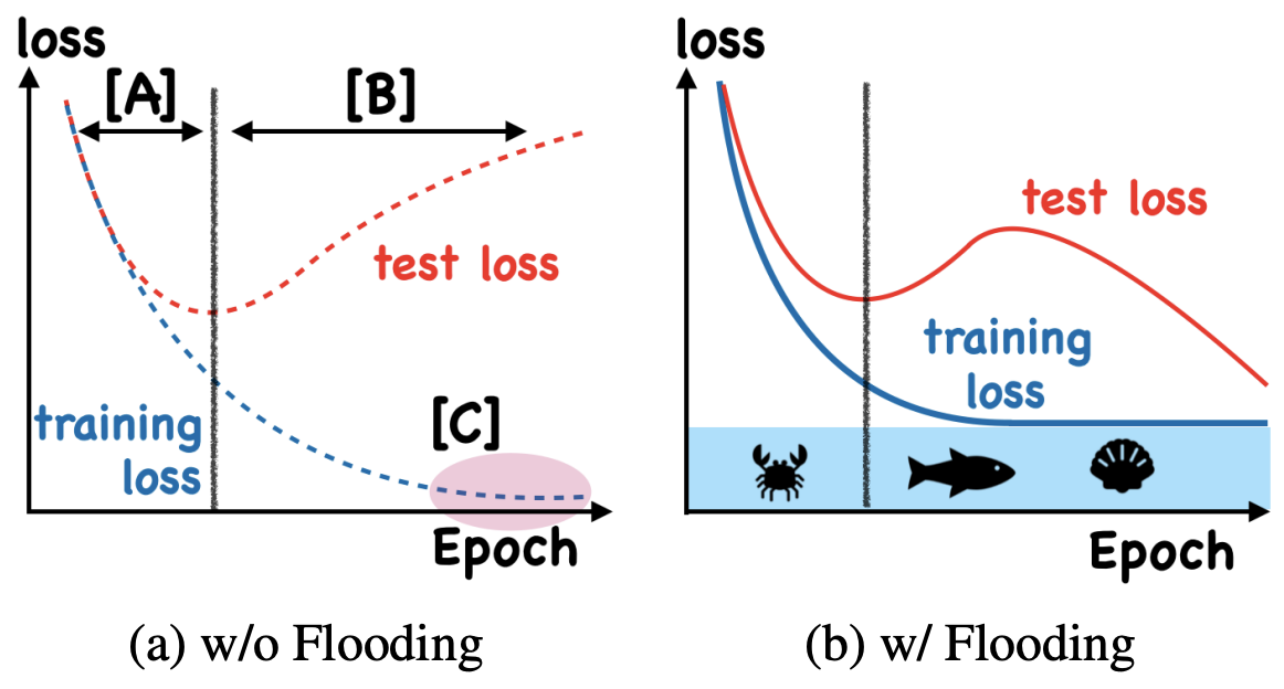
BTW, look at that deep-double descent!

[1] T. Ishida, et al. Do We Need Zero Training Loss After Achieving Zero Training Error? Arxiv: 2002.08709