Machine Learning for Engineering

Neural Networks: Model Bias

Instructor: Daning Huang

$$ \newcommand\ppf[2]{\dfrac{\partial #1}{\partial #2}} \newcommand\norm[1]{\left\Vert#1\right\Vert} \newcommand{\bR}{\mathbb{R}} \newcommand{\cD}{\mathcal{D}} \newcommand{\cL}{\mathcal{L}} \newcommand{\cN}{\mathcal{N}} \newcommand{\vF}{\mathbf{F}} \newcommand{\vH}{\mathbf{H}} \newcommand{\vI}{\mathbf{I}} \newcommand{\vK}{\mathbf{K}} \newcommand{\vL}{\mathbf{L}} \newcommand{\vM}{\mathbf{M}} \newcommand{\vO}{\mathbf{O}} \newcommand{\vQ}{\mathbf{Q}} \newcommand{\vV}{\mathbf{V}} \newcommand{\vW}{\mathbf{W}} \newcommand{\vb}{\mathbf{b}} \newcommand{\vf}{\mathbf{f}} \newcommand{\vh}{\mathbf{h}} \newcommand{\vm}{\mathbf{m}} \newcommand{\vx}{\mathbf{x}} \newcommand{\vy}{\mathbf{y}} $$

TODAY: Neural Networks

• Model biases
• An illustrative example
• Some additional perspectives

General Discussion

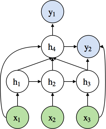
FAQ: Does a neural network have to be always layer-structured?

• No. It can be any directed acyclic graph (DAG).
• Example of a complex neural network

FAQ: Can we define any arbitrary layers?

• We can define any layer as long as it is differentiable.
  • When it is not differentiable, we can make it approximately so.
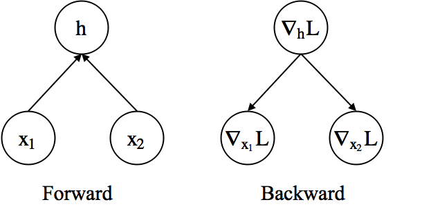
• Example) Addition layer
  • Forward: $\textbf{h} = \textbf{x}_1 + \textbf{x}_2$
  • Backward
    • $\nabla_{\textbf{x}_1}\mathcal{L} = \nabla_{\textbf{h}}\mathcal{L}\nabla_{\textbf{x}_1}\textbf{h}=\nabla_{\textbf{h}}\mathcal{L}$
    • $\nabla_{\textbf{x}_2}\mathcal{L} = \nabla_{\textbf{h}}\mathcal{L}\nabla_{\textbf{x}_2}\textbf{h}=\nabla_{\textbf{h}}\mathcal{L}$

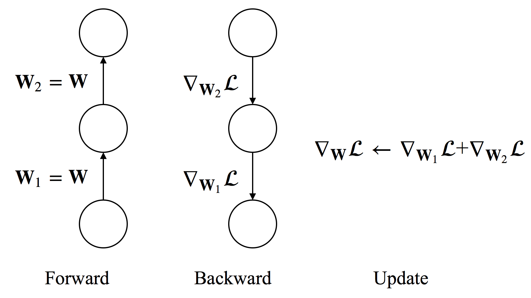
FAQ: How to handle shared weights?

• To constrain $W_1=W_2=W$, we need $\Delta W_1 = \Delta W_2$.
• Compute $\nabla_{W_1}\mathcal{L}$ and $\nabla_{W_2}\mathcal{L}$ separately.
• Use $\nabla_{W}\mathcal{L}=\nabla_{W_1}\mathcal{L}+\nabla_{W_2}\mathcal{L}$ to update the shared weight.
• In practice, we accumulate gradients to the shared memory space for $\nabla_{W}\mathcal{L}$ during back-propagation.
• Weight sharing is used in convolutional neural networks and recurrent neural networks.

What is "deep" neural network?

• If we have to given a definition...
• A neural network is considered to be deep if it has more than two (non-linear) hidden layers.
• Higher layers extract more abstract and hierarchical features.

• Difficulties in training deep neural networks
  • Easily overfit (The number of parameters is large)
  • Hard to optimize (highly non-convex optimization)
  • Computationally expensive (many matrix multiplications)
• Recent Advances
  • Large-scale dataset (e.g., 1M images in ImageNet, PB text for ChatGPT)
  • Better regularization (e.g., Dropout, Spectral)
  • Better optimization (e.g., Adam family, Muon)
  • Better hardware (GPU/TPU for matrix computation)

"Bias" of a Model

The FAQ basically says we can design any parametrized model of any architecture.

But we would want the family of models to be compatible with the problem at hand.

For example, the model should

• Capture temporal correlation for time series.
• Generate localized features for object detection in images.
• Preserve symmetry of the original problem. (e.g., if we fit an odd function, the NN should be odd too)
• Satisfy any physics-based relations that are already known.
• etc.

The level of model-problem compatibility is referred to as model bias.

Not to be confused with the bias-variance trade-off

Biases

There are (at least) four types of biases: observational, learning, inductive, and physics.

Refs: Battaglia2018, Karniadakis2021

To make it more tangible, suppose we want to fit a simple model for a nonlinear spring $$ F = k_1 x + k_2 x^3 $$ given data of $(x_i,F_i)$.

• Physical knowledge tells us that the model should be an odd function.

Observation Bias

• No special structure on the model.
• Manipulate the data so that it satisfies our knowledge
  • For a data point $(x_i,F_i)$, make sure $(-x_i,-F_i)$ is also a data point.
  • Or, sample strategically to achieve the same effect
• Within the range of (augmented) data, the learned model is approximately an odd function.

Cons: Higher training cost for larger dataset; only approximation

Learning Bias

• No special structure on the model or data.
• Design special losses to enforce the model form.
  • Add a penalty $L(x) = f(x)+f(-x)$
  • $f(x)$ gets penalized when it is not odd

• One more example: "physics-informed" neural network

  • Want solution to a PDE $u_{xx}+u_{yy}=0$.
  • Define a network $u^*(x,y)$ and drive a loss $||u^*_{xx}+u^*_{yy}||$ to zero.
  • (Technically we also need losses on boundary conditions)

• More on these models in this module.

Inductive Bias

• Place structure on the model to enforce known knowledge.
  • Given any model $\hat{f}(x)$, define $f(x) = \hat{f}(x)-\hat{f}(-x)$ as our final model.
  • $f(x)$ is always odd.

• One more example: Say we want the output to be a $3\times 3$ rotation matrix $R$.
  • Need $|R|=1$, so simply outputing a $3\times 3$ array would not work.
  • Instead we learn a vector $x=[x_1,x_2,x_3]$, and for any $x$, $\exp(\hat{x})$ is a rotation matrix $$ \hat{x} = \begin{bmatrix} 0 & -x_3 & x_2 \\ x_3 & 0 & -x_1 \\ -x_2 & x_1 & 0 \end{bmatrix} $$

Physics Bias

• Embed physics-based model into the model.
  • Suppose we know a baseline relation $F\approx k^* x$, $k^*$ known
  • Define model as $F=k^* x + \hat{f}(x)$, and learn $\hat{f}$ instead of the entire $F$.

• One more example: Constitutive relations for elasticity
  • $\nabla\cdot \sigma(\epsilon)=F$, $F$ force, $\sigma$ stress, $\epsilon$ strain
  • We keep the equation in the model and just learn $\sigma(\epsilon)$

Classical Deep Architectures

• Convolutional Neural Network (CNN)
  • Widely used for image modeling
  • e.g. object recognition, segmentation, vision-based reinforcement learning problems
  • e.g. flow analysis and modeling (i.e. thinking the flow field as 2D/3D images)
• Recurrent Neural Network (RNN)
  • Widely used for sequential data modeling
  • e.g. machine translation, image caption generation
  • e.g. time series analysis and forecasting, nonlinear dynamics

These are mainly the cases of inductive bias.

An Illustrative Example

Let's fit a NN to predict the area $A$ of a triangle given its edge lengths $(a,b,c)$.

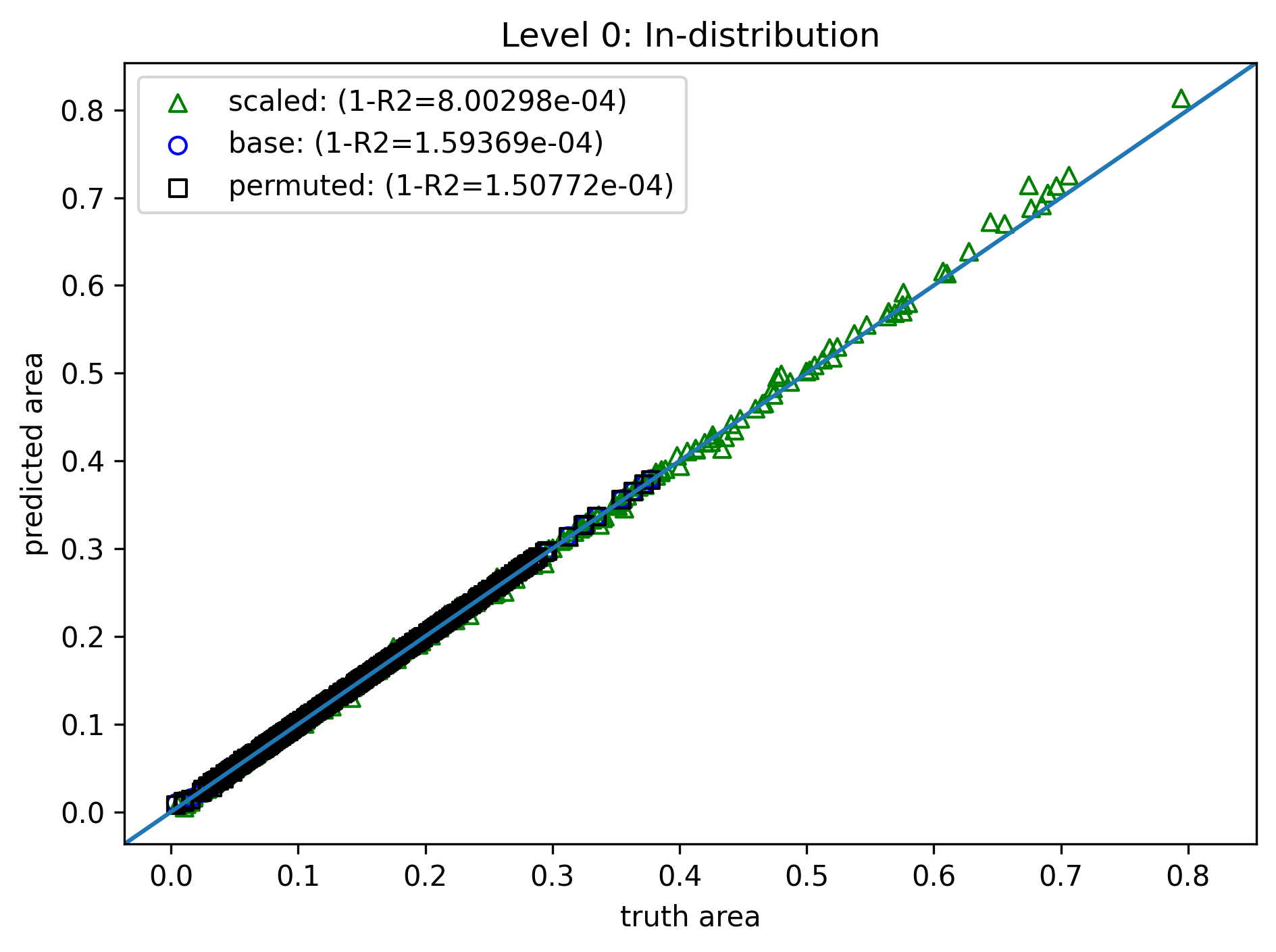
Level 0: Do nothing

• Model: 3 hidden layers, 128 neurons each
• Training data: 4000 samples of $\{(a_i,b_i,c_i),A_i\}_{i=1}^N$, length range $(0.2, 1.0)$
• Loss: Simple RMSE $$ \mathcal{L}(\theta) = \sum_{i=1}^N \|A_i - f(a_i,b_i,c_i)\|^2 $$
• Training: 2000 epoch (no validation for simplicity), Adam optimizer

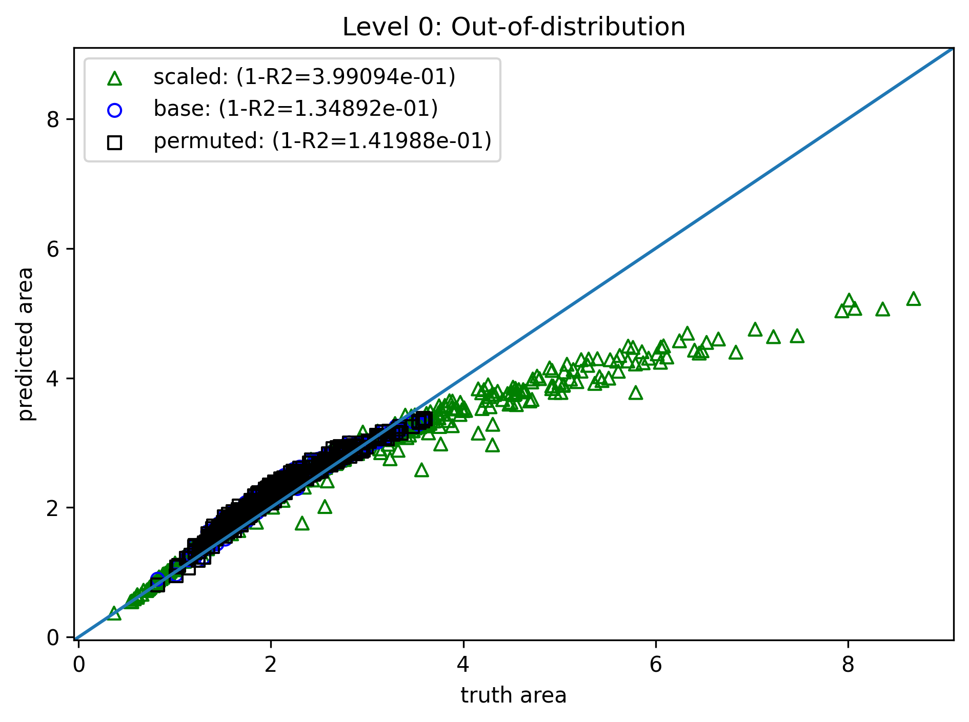
Test data variation:

• "base": 4000 samples, same length distribution
• "permuted": Edge order permuted - the output should be the same
• "scaled": Edges are uniformly scaled, scaling factor $s$ range $(0.6,1.7)$ - the output should scale by $s^2$

Two test datasets:

• In distribution: length range $(0.2, 1.0)$, same as training.
• Out of distribution: length range $(1.5, 3.0)$, i.e., entirely unseen in training.

Deviation starts as edge lengths increase.

Completely off!

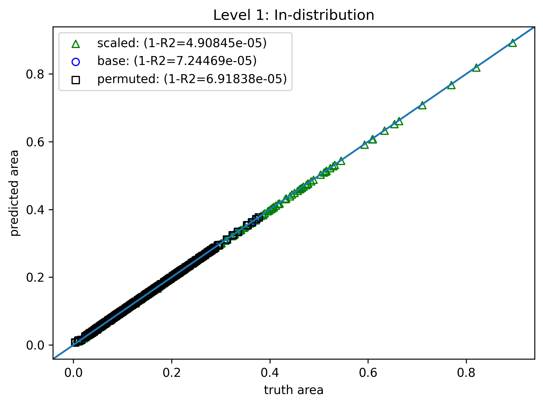
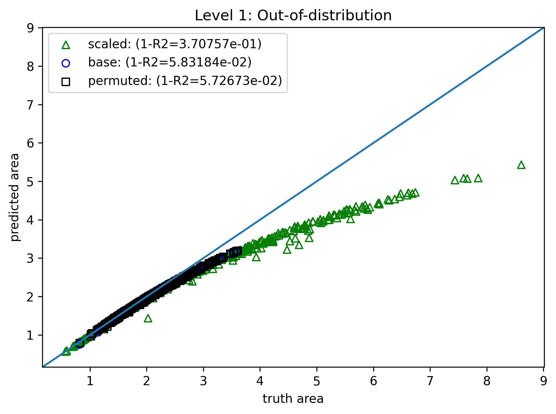
Level 1: Observation Bias

• Same model, training method, and loss
• Training data: 4000 samples of $\{(a_i,b_i,c_i),A_i\}_{i=1}^N$, length range $(0.2, 1.0)$
• Data augmentation: For each sample,
  • Permutation produces 5 more samples: $\{(a_i,c_i,b_i),A_i\}_{i=1}^N$, $\{(c_i,a_i,b_i),A_i\}_{i=1}^N$, etc.
  • Scaling produces 1 more sample: $\{(sa_i,sc_i,sb_i),s^2A_i\}_{i=1}^N$ ($s$ randomly chosen).

• In-distribution is nearly perfect, but OOD is still off.
• Training cost increased from 16s to 42s (b/c more data).

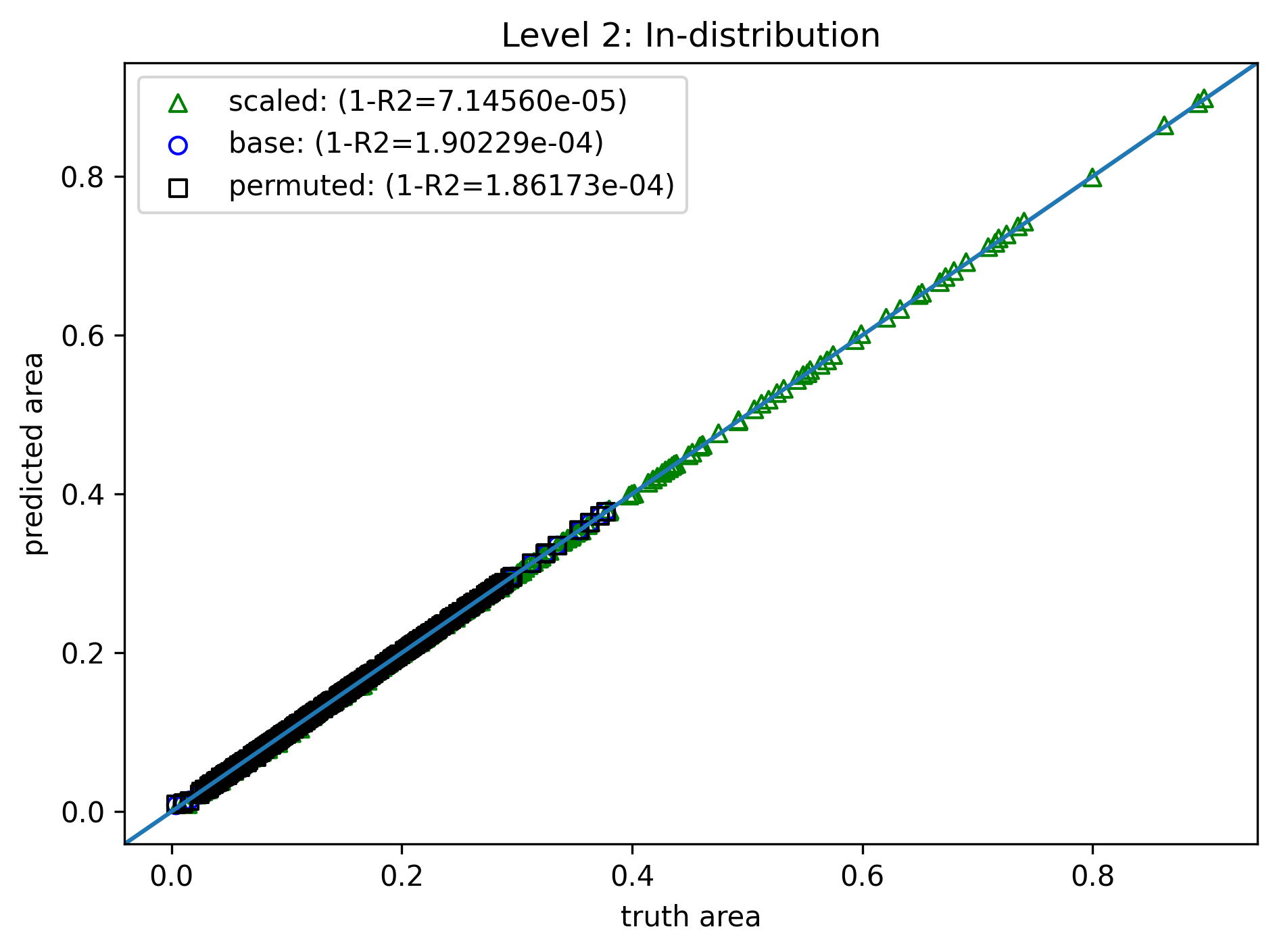
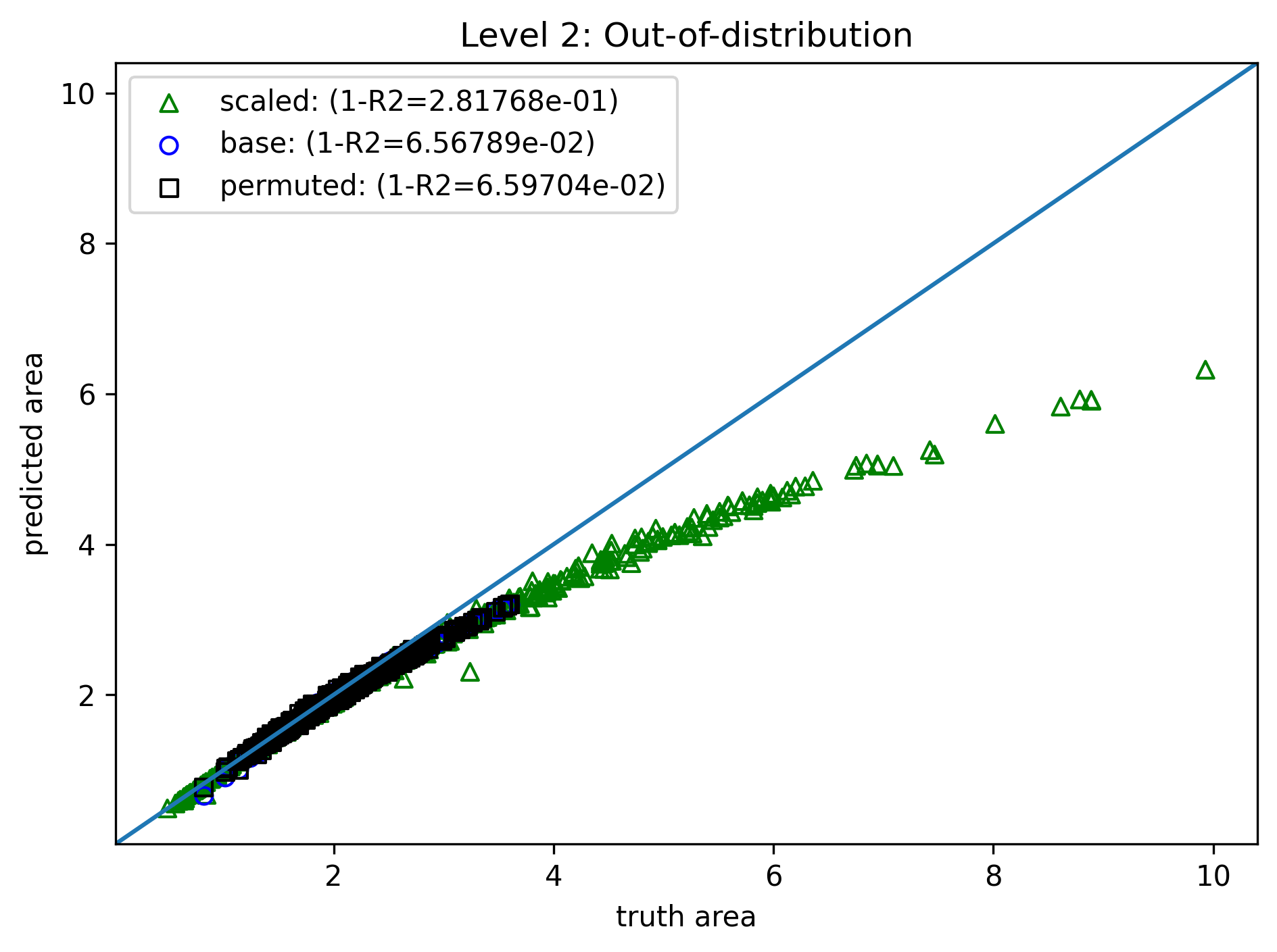
Level 2: Learning Bias

• Same model, training method, and data
• Modify the loss
  • Permutation penalty $$ \mathcal{L}_p(\theta) = \sum_{i=1}^N \|A_i - f(a_i,c_i,b_i)\|^2 + \sum_{i=1}^N \|A_i - f(c_i,a_i,b_i)\|^2 + \cdots $$
  • Scaling penalty, for random $s$ $$ \mathcal{L}_s(\theta) = \sum_{i=1}^N \|s^2A_i - f(sa_i,sc_i,sb_i)\|^2 $$
  • Total loss, with user-specified weights $$ \mathcal{L}_{tot} = \mathcal{L} + w_p \mathcal{L}_p + w_s \mathcal{L}_s $$

• Similar to level 1
• Training cost further increased to 66s! (extra backpropagation in penalty terms)

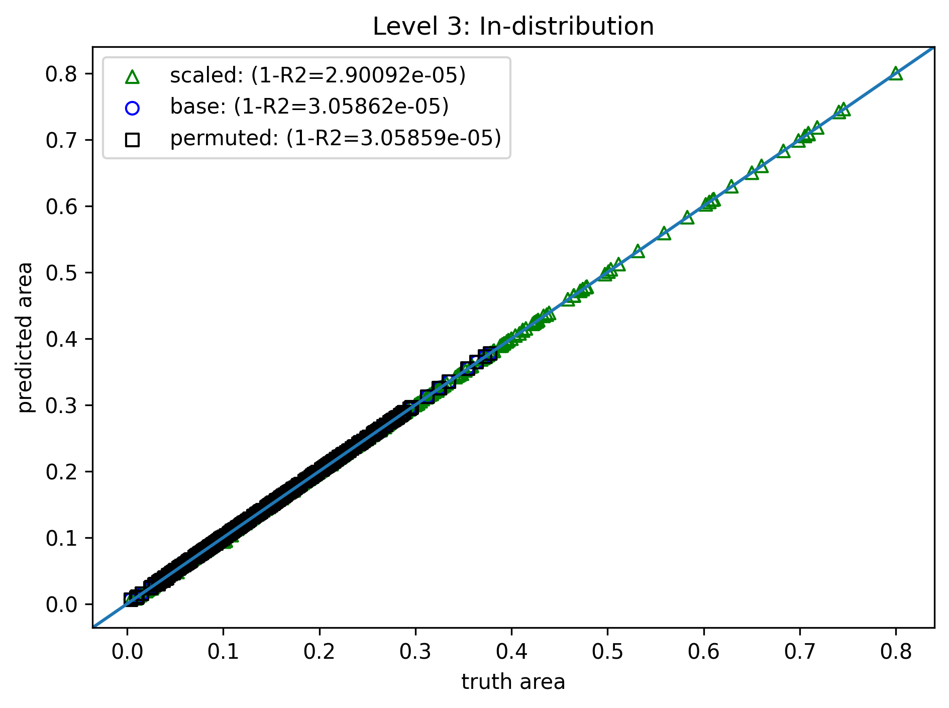
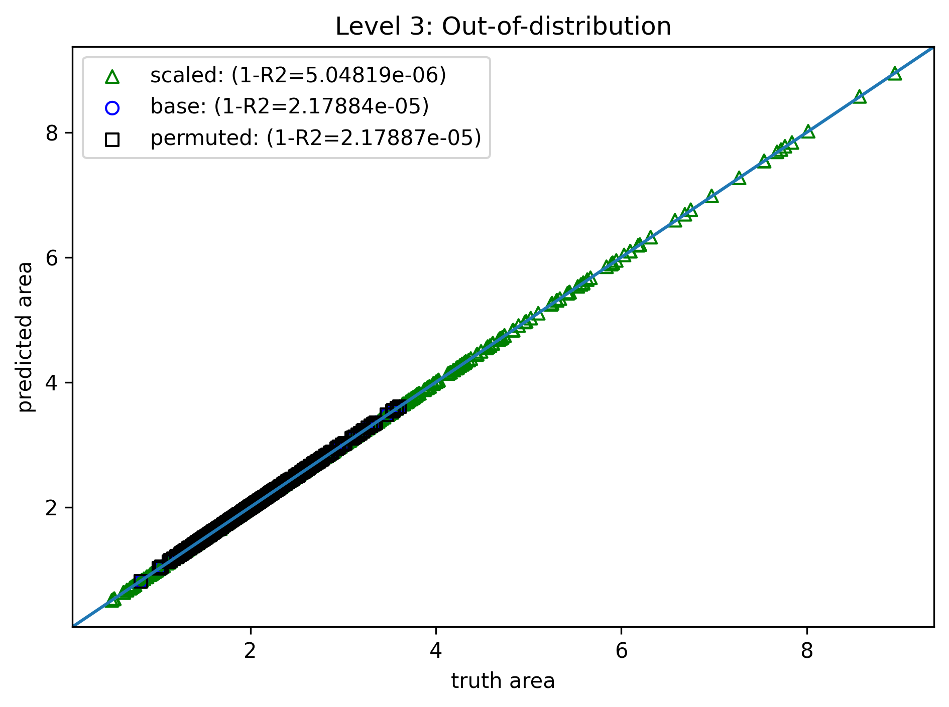
Level 3: Inductive Bias

• Same training method, data, and loss
• Modify the model for guaranteed permutation and scaling symmetries
  • Normalize: $(\tilde{a}, \tilde{b}, \tilde{c}) = (a,b,c) / s$, $s=a+b+c$
  • Sort: $(\tilde{a}, \tilde{b}, \tilde{c}) \rightarrow (\bar{a}, \bar{b}, \bar{c})$ (e.g., high to low)
  • MLP evaluation: $\bar{A} = f(\bar{a}, \bar{b}, \bar{c})$
  • Scaling: $A=s^2\bar{A}$

• Now both ID and OOD are nearly perfect!
• Train cost reduces to 16s again (same as level 0)

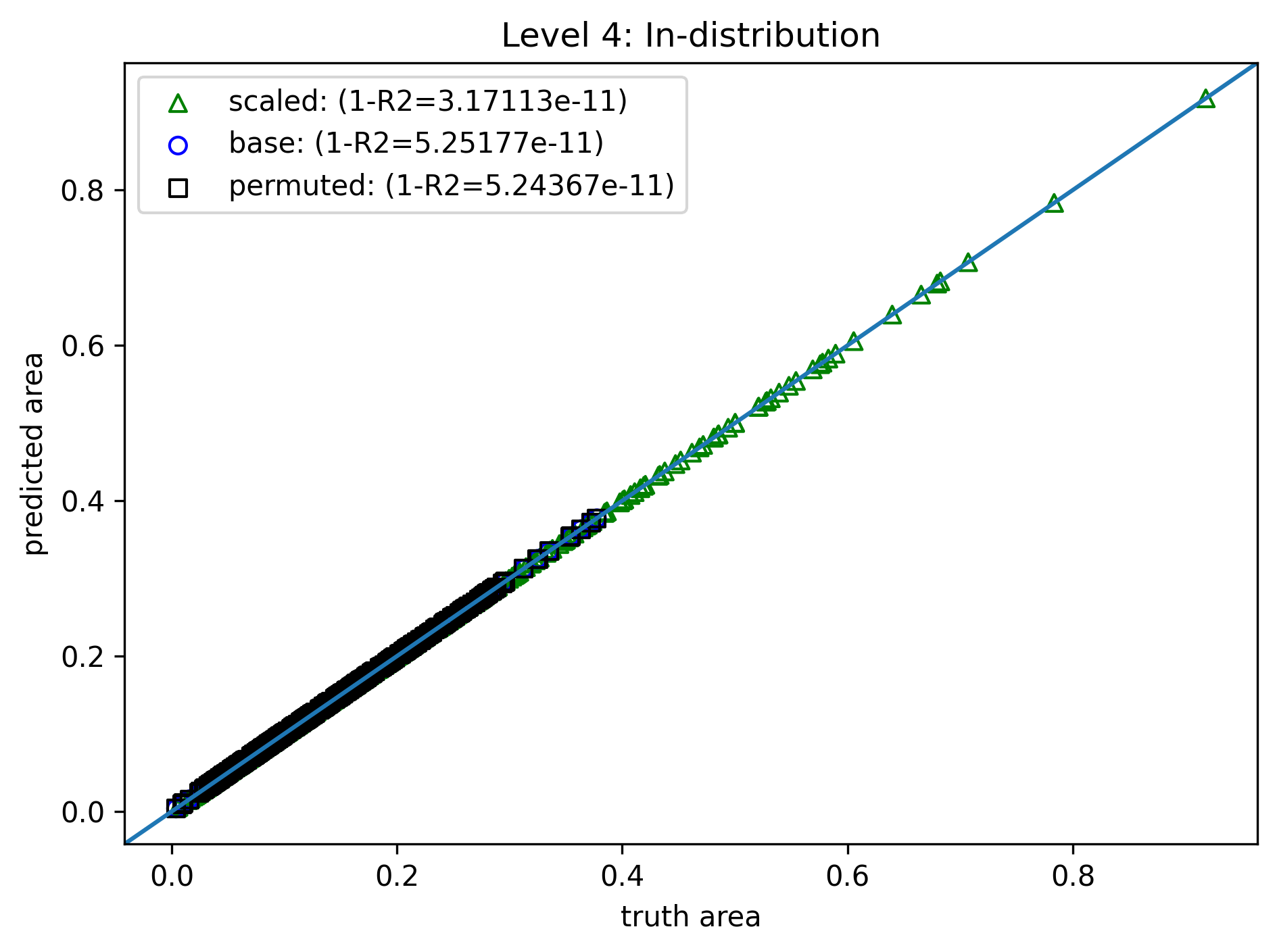
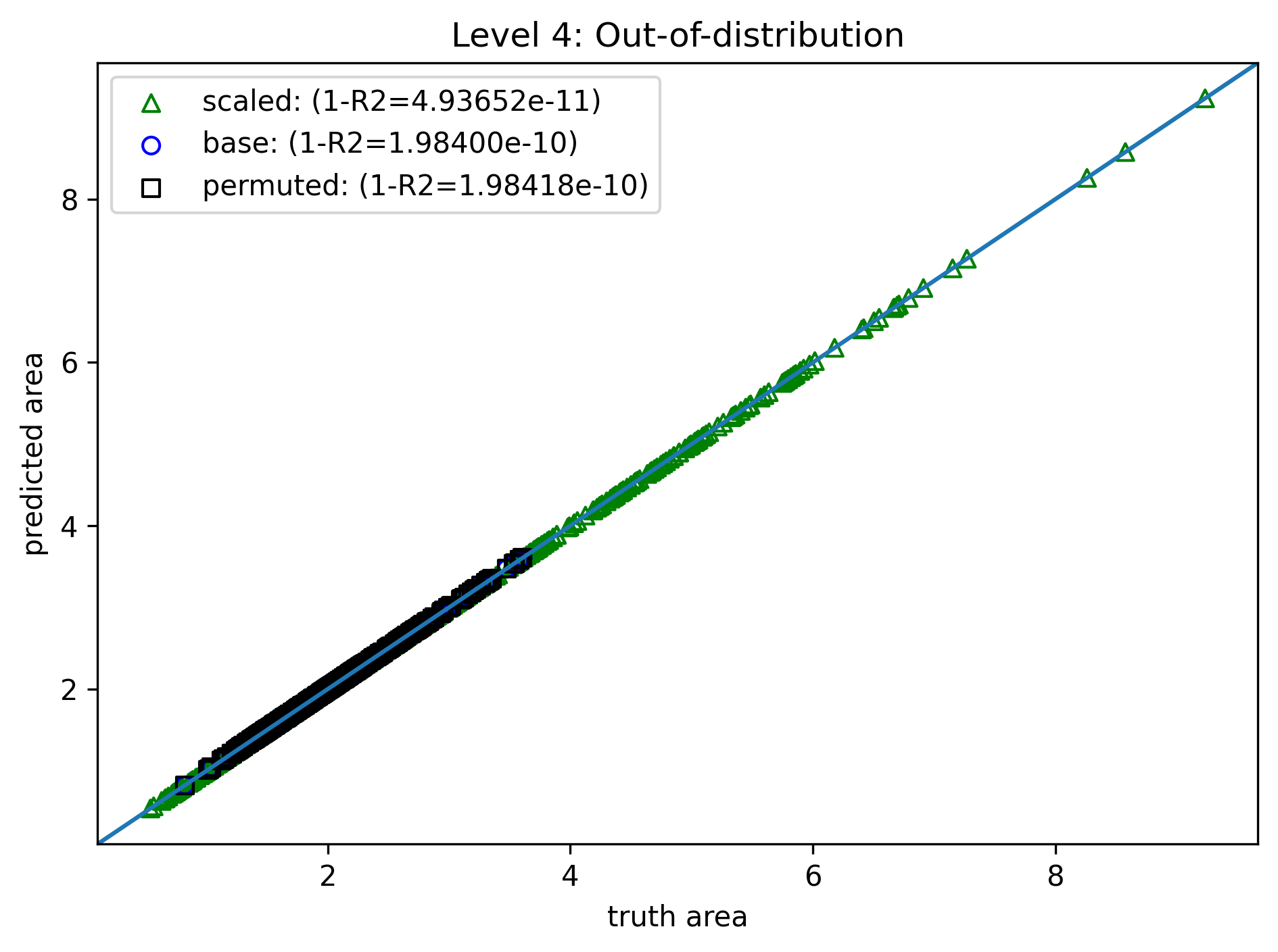
Level 4: "Physics" Bias

• Same training method, data, and loss
• Modify the model further by domain knowledge - only one parameter $C$ to fit $$ f(a,b,c) = C\sqrt{(a+b+c)(a+b-c)(a-b+c)(-a+b+c)} $$

The detailed reasoning is two slides later

• Perfect fit
• A few millisec to train

Reasons for choosing the particular model form.

1. In the extreme cases $c=a+b$, $b=a+c$, $a=b+c$, area should be 0; so we guess $f(a,b,c)$ contains a factor of $(a+b-c)(a-b+c)(-a+b+c)$.
2. Area has dimension $\text{length}^2$, but the factor is $\text{length}^3$; so we guess $$ f(a,b,c)^2 = g(a,b,c)(a+b-c)(a-b+c)(-a+b+c) $$ where $g(a,b,c)$ has dimension $\text{length}$
3. There is permutation symmetry, so the simplest choice is $g(a,b,c) = C_1 (a+b+c)$.
4. Hence we obtain the previously assumed form. Note it satisfies scaling symmetry too.

One More Perspective

Consider the optimization of a loss $\mathcal{L}$ with a model $f$, given parameter $\theta$, $$ \mathcal{L} = \mathcal{L}(f(\theta)) $$

If the optimized model does not perform well, it usually means

• Gradient is zero at unfavorable places
• and we are stuck in one of them

When is gradient zero?

The gradient can be viewed as an inner product,

$$ \frac{\partial \mathcal{L}}{\partial \theta} = \left\langle \left. \frac{\partial \mathcal{L}}{\partial F} \right|_{F = f(\theta)}, \; \frac{\partial f(\theta)}{\partial \theta} \right\rangle $$

where $F = f(\theta)$ highlights the model evaluation at the current iterate $\theta$.

Then the zero gradient implies the orthogonality between $$ \frac{\partial \mathcal{L}}{\partial F} \quad \text{and} \quad \frac{\partial f(\theta)}{\partial \theta} $$

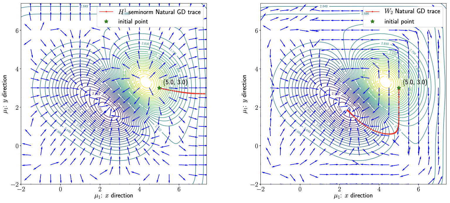
Fixing orthogonality

If the gradient is not supposed to be zero, we can try modifying

• the loss $\mathcal{L}$ (e.g., the observation and learning biases)
• the model $f$ (e.g., the inductive and physics biases)
• the inner product itself (e.g., the learning bias)

Example

• Left: diverge due to inappropriate loss
• Right: changing loss gives the correct gradient to the basin SISC2023