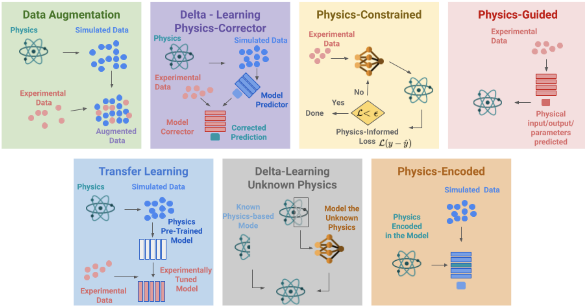
In this lecture we will discuss one basic physics-informed NN
- This belongs to the "Physics-Constrained" category above
- Not going to cover things like operator learning (e.g., DeepONet and FNO) in this category
Physics-Informed Neural Networks (PINNs)
- Solves differential equations
- Incorporates physics via learning bias.
- Not new: as early as 1994: Dissanayake, M. W. M. G., and Nhan Phan‐Thien. "Neural‐network‐based approximations for solving partial differential equations." communications in Numerical Methods in Engineering 10.3 (1994): 195-201.
- Revival around 2017: Raissi, Maziar, Paris Perdikaris, and George Em Karniadakis. "Physics informed deep learning (part i): Data-driven solutions of nonlinear partial differential equations." arXiv preprint arXiv:1711.10561 (2017).
- A relatively recent summary (2021): Lu, Lu, et al. "DeepXDE: A deep learning library for solving differential equations." SIAM Review 63.1 (2021): 208-228.
Model Problem
For unknown function $u$ with coordinates $z$, $$ \begin{align} \cF[u] &= f(z)\quad z\in\Omega \\ \cB[u] &= b(z)\quad z\in\partial\Omega \end{align} $$ where Eq. (1) is the differential equation and Eq. (2) are the boundary/initial conditions.
Example PDE
On domain $\Omega=[0,1]\times [0,1]$, coordinates $z=[x,y]$ $$ \begin{align*} u_{xx}-u_{yyyy} &= (2-x^2)\exp(-y) \\ u_{yy}(x,0)=x^2,&\ u_{yy}(x,1)=x^2/e \\ u(x,0)=x^2,&\ u(x,1)=x^2/e \\ u(0,y)=0,&\ u(1,y)=\exp(-y) \end{align*} $$
The solution is $$ u(x,y)=x^2\exp(-y) $$
Core Idea
- Nested automatic differentiation to obtain higher-order derivatives
- Represent the solution $u(z)$ as a neural network
- Express the equations in the loss
Example
Denote a neural network $\tilde{u}(z;\theta)$, where $z$ is input/coordinate, and $\theta$ is model parameter.
A learning framework can give us
- $\tilde{u}_\theta$: Most common, as needed for training
- $\tilde{u}_z$: Less common, but certainly possible
- $\tilde{u}_{\theta\theta}$: Rarely done, but possible - back-propagate twice
- $\tilde{u}_{zz}$, $\tilde{u}_{zzz}$, etc.: Same - possible
# Note the nested gradients
def gradients(u, x, order=1):
    if order == 1:
        return torch.autograd.grad(
            u, x, grad_outputs=torch.ones_like(u),
            create_graph=True, only_inputs=True)[0]
    else:
        return gradients(gradients(u, x), x, order=order - 1)
Physics-Informed Losses
For a function $\tilde{u}$ to be a solution to a given PDE, we want $$ \begin{align*} R_F(\tilde{u}) &= \cF[\tilde{u}] - f(z) = 0\quad z\in\Omega \\ R_B(\tilde{u}) &= \cB[\tilde{u}] - b(z) = 0\quad z\in\partial\Omega \end{align*} $$ Regardless of whether $\tilde{u}$ is an analytical function, a numerical solution, or a neural network!
In other words, define
- Loss for equation: $$ \cL_F(\theta) \equiv \norm{R_F(\tilde{u})}^2 = \int_\Omega \norm{\cF[\tilde{u}] - f(z)}^2 dz $$
- Loss for BCs/ICs: $$ \cL_B(\theta) \equiv \norm{R_B(\tilde{u})}^2 = \int_{\partial\Omega} \norm{\cB[\tilde{u}] - b(z)}^2 dz $$
If we minimize $\cL(\theta) = \cL_F(\theta) + \cL_B(\theta)$, then $\tilde{u}$ approximately solves the PDE!
Back to Example PDE
First define a generic neural network - no special biases at all
class MLP(torch.nn.Module):
    def __init__(self):
        super(MLP, self).__init__()
        self.net = torch.nn.Sequential(
            torch.nn.Linear(2, 32),
            torch.nn.Tanh(),
            torch.nn.Linear(32, 32),
            torch.nn.Tanh(),
            torch.nn.Linear(32, 32),
            torch.nn.Tanh(),
            torch.nn.Linear(32, 32),
            torch.nn.Tanh(),
            torch.nn.Linear(32, 1)
        )
    def forward(self, x):
        return self.net(x)
Creating losses
The differential equation was $$ u_{xx}-u_{yyyy} = (2-x^2)\exp(-y),\quad \Omega=[0,1]\times[0,1] $$
Suppose we sample the domain $\Omega$ at a few points $\{(x_i,y_i)\}_{i=1}^N$, and define $$ \cL_F(\theta) = \int_\Omega \norm{\cF[\tilde{u}] - f(z)}^2 dz \approx \frac{1}{N}\sum_{i=1}^N \norm{ \tilde{u}_{i,xx} - \tilde{u}_{i,yyyy} - (2-x_i^2)\exp(-y_i) }^2 $$ where $\tilde{u}_{i,xx}$ is $\tilde{u}_{xx}$ evaluated at $(x_i,y_i)$
def interior(n=1000):   # Sample 1000 points
    x = torch.rand(n, 1)
    y = torch.rand(n, 1)
    cond = (2 - x ** 2) * torch.exp(-y)
    return x.requires_grad_(True), y.requires_grad_(True), cond

loss = torch.nn.MSELoss()
def l_interior(u):      # Define the loss for equation
    x, y, cond = interior()
    uxy = u(torch.cat([x, y], dim=1))
    # loss(Prediction, Truth)
    return loss(gradients(uxy, x, 2) - gradients(uxy, y, 4), cond)
Then for the BCs - the first one was $$ u_{yy}(x,0)=x^2,\quad x\in[0,1] $$ With samples $\{(x_i,0)\}_{i=1}^M$ on the boundary: $$ \cL_{B1}(\theta) = \int_{\partial\Omega} \norm{\cB[\tilde{u}] - b(z)}^2 dz \approx \frac{1}{M} \sum_{i=1}^M \norm{\tilde{u}_{i,yy}-x_i^2}^2 $$
def down_yy(n=100):
    x = torch.rand(n, 1)
    y = torch.zeros_like(x)
    cond = x ** 2
    return x.requires_grad_(True), y.requires_grad_(True), cond

def l_down_yy(u):
    x, y, cond = down_yy()
    uxy = u(torch.cat([x, y], dim=1))
    return loss(gradients(uxy, y, 2), cond)
We can continue to write the losses for the other BCs, e.g., which one is this -
def up_yy(n=100):
    x = torch.rand(n, 1)
    y = torch.ones_like(x)
    cond = x ** 2 / torch.e
    return x.requires_grad_(True), y.requires_grad_(True), cond

def l_up_yy(u):
    x, y, cond = up_yy()
    uxy = u(torch.cat([x, y], dim=1))
    return loss(gradients(uxy, y, 2), cond)
The rest BCs are skipped for conciseness.
Then we simply train the network with the sum of losses: $$ \cL(\theta) = \cL_F(\theta) + \sum_{i=1}^6 \alpha_i\cL_{Bi}(\theta) $$ Technically we can use a weighted sum with $\alpha_i\neq 1$
- Or with $\alpha_i=1$ but more samples in regions of more interest
- Or a vanilla sum of squares is somewhat self-adaptive
Example cont'd
Training & Results
u = MLP()
opt = torch.optim.Adam(params=u.parameters())
N, ls = 2000, []
for i in range(N):      # Standard and basic training
    opt.zero_grad()
    l1 = l_interior(u)
    l2 = l_up_yy(u) + l_down_yy(u) + l_up(u) + l_down(u) + l_left(u) + l_right(u)
    l = l1+l2
    l.backward()
    opt.step()
    ls.append([l1.detach().numpy(), l2.detach().numpy()])
    if i % 50 == 0:
        print(f"Step {i}/{N}: {l}")
Step 0/2000: 2.179628372192383
Step 50/2000: 0.32033467292785645
Step 100/2000: 0.20419979095458984
Step 150/2000: 0.15413124859333038
Step 200/2000: 0.09876691550016403
Step 250/2000: 0.07022074609994888
Step 300/2000: 0.044294316321611404
Step 350/2000: 0.04057040065526962
Step 400/2000: 0.022583819925785065
Step 450/2000: 0.01602921634912491
Step 500/2000: 0.009486999362707138
Step 550/2000: 0.004785760305821896
Step 600/2000: 0.0022005755454301834
Step 650/2000: 0.001665947842411697
Step 700/2000: 0.0009323493577539921
Step 750/2000: 0.0006346203153952956
Step 800/2000: 0.0005713048158213496
Step 850/2000: 0.00039342950913123786
Step 900/2000: 0.0003619924536906183
Step 950/2000: 0.0003511778195388615
Step 1000/2000: 0.00025024267961271107
Step 1050/2000: 0.0003133229911327362
Step 1100/2000: 0.0007971076411195099
Step 1150/2000: 0.0002571406657807529
Step 1200/2000: 0.0007301169098354876
Step 1250/2000: 0.00046473758993670344
Step 1300/2000: 0.000545755960047245
Step 1350/2000: 0.0003433202509768307
Step 1400/2000: 0.0003754120843950659
Step 1450/2000: 0.0003412280639167875
Step 1500/2000: 0.00024082761956378818
Step 1550/2000: 0.0002805497497320175
Step 1600/2000: 0.0010911432327702641
Step 1650/2000: 0.0004066715482622385
Step 1700/2000: 0.0002538096741773188
Step 1750/2000: 0.0002924928558059037
Step 1800/2000: 0.0003928612277377397
Step 1850/2000: 0.00019409907690715045
Step 1900/2000: 0.00044656568206846714
Step 1950/2000: 0.0002111586363753304
L = np.array(ls).T
f = plt.figure(figsize=(10,5))
plt.semilogy(L[0], 'k--', label="Equation loss")
plt.semilogy(L[1], 'r:', label="BC loss")
plt.semilogy(L[0]+L[1], 'b-', label="Total loss")
plt.legend()
plt.xlabel("Iterations")
plt.ylabel("Loss");
f, ax = plt.subplots(ncols=3, sharey=True, figsize=(12,4))
f.subplots_adjust(bottom=0.1, top=0.9, left=0.1, right=0.9, wspace=0.02, hspace=0.02)
ax2 = f.add_axes([0.95, 0.05, 0.05, 0.9])
cs = ax[0].contourf(xx, yy, u_true)
ax[1].contourf(xx, yy, u_pred, levels=cs.levels)
ax[2].contourf(xx, yy, np.abs(u_true-u_pred), levels=cs.levels)
ax[0].set_title("Truth")
ax[1].set_title("Prediction")
ax[2].set_title("Error")
f.colorbar(cs, cax=ax2);
err = np.linalg.norm(u_pred-u_true) / np.linalg.norm(u_true)
print(f"Max abs error is: {err}")
Max abs error is: 0.006881872657686472
Going beyond basics
Inverse Problem
- Only know partial measurements
- Add a regular loss on data samples to PINN
- Recover physically consistent full measurements

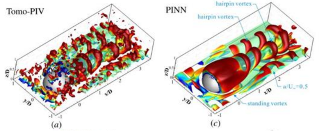
Example: Wang, Hongping, Yi Liu, and Shizhao Wang. "Dense velocity reconstruction from particle image velocimetry/particle tracking velocimetry using a physics-informed neural network." Physics of Fluids 34.1 (2022): 017116.
Domain Complexity
- Rectangular or circular domain is easy to sample - how about complex geometry?
- One could do domain decomposition

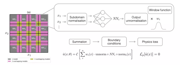
Example: Moseley, Ben, Andrew Markham, and Tarje Nissen-Meyer. "Finite Basis Physics-Informed Neural Networks (FBPINNs): a scalable domain decomposition approach for solving differential equations." arXiv preprint arXiv:2107.07871 (2021).
Higher-order Derivatives
- High-order derivatives are really slow due to multiple back-props
- Use "weak form" to reduce the derivative order [1]
- Or use finite difference methods to approximate some of the derivatives [2]

[1] Lyu, Liyao, et al. "MIM: A deep mixed residual method for solving high-order partial differential equations." Journal of Computational Physics (2022): 110930.
[2] Chen, Yuntian, et al. "Theory-guided hard constraint projection (HCP): A knowledge-based data-driven scientific machine learning method." Journal of Computational Physics 445 (2021): 110624.
Typical concerns:
- Training speed
- Convergence guarantees
- Accuracy, esp. resolution of multiple scales
- Generalization to unseen scenarios
Still active research area...
A practical reference: An Expert's Guide to Training Physics-informed Neural Networks
