Machine Learning for Engineering

Introduction: Posing the Problem and the Scope

Instructor: Daning Huang

$$ \newcommand{\norm}[1]{\left\lVert{#1}\right\rVert} \newcommand{\R}{\mathbb{R}} \renewcommand{\vec}[1]{\mathbf{#1}} \newcommand{\X}{\mathcal{X}} \newcommand{\D}{\mathcal{D}} \newcommand{\cL}{\mathcal{L}} $$

Definitions

Consider a generic model $$ \hat{y} = f(x,\theta) $$ where

• $f$ model
• $x$ input
• $\theta$ parameter
• $\hat{y}$ predicted output

Given a dataset of $N$ samples $$ \D = \{(x_i, y_i)\}_{i=1}^N $$ we minimize a loss $$ \min_\theta \cL(y,\hat{y}) $$

Example 1

The simplest model is perhaps linear regression: $$ f(x,\theta) = \theta_0 + \theta_1 x_1 + \cdots + \theta_m x_m \equiv \theta^T\phi(x) $$ with a squared loss $$ \cL(y,\hat{y}) = \sum_{i=1}^N \norm{y_i-\theta^T\phi(x_i)}^2 $$ For this one we have closed-formed solution.

Example 2

Consider a general non-linear dynamical system: $$ \begin{align*} \dot{x} &= f(x,t,u;\mu) + d,\quad x(0)=x_0 \\ y_k &= g(x_k,t_k,u_k;\mu) + \epsilon \end{align*} $$

• $x$: State vector, possibly very high dimensional
• $y$: Observation vector, possibly also high-dim and over discrete time
• $t$: Time, there could be multiple time scales
• $x_0$: Initial conditions, sensitivity to $x_0$ - chaos?
• $u$: Control inputs
• $\mu$: System parameters
• $d$, $\epsilon$: Disturbance, Noise

Given

• Trajectories $D=\{(t_i,u_i,\mu_i,y_i)\}_{i=1}^N$
• Possibly also knowledge about the problem
  • Physical properties: conservativeness, stability, etc.
  • Part of governing equations

Identify $$ \begin{align*} \dot{x} &= \hat{f}(x,t,u;\mu),\quad x(0)=x_0 \\ y_k &= \hat{g}(x_k,t_k,u_k;\mu) \end{align*} $$

• To reproduce the given data and generalize to unseen data
• If possible provide an error estimate on the prediction

Challenge comes in when we go for more complex models, e.g., "deep" models. Possible complexities:

• Input/Output, $x,y$
  • Images, Audio, Graph, text
  • Missing data
  • Data noise
  • etc.

• Model form, $f$
  • Multi-layer perceptron
  • Differential equations
  • Embedded optimization
  • etc.

• Loss, $\cL$
  • Parametric sparsity
  • Physics-informed losses
  • Lipschitz constant
  • etc.

• Difficulties in learning deep models
  • Easily overfit ... or not? (large number of parameters)
  • Hard to optimize (highly non-convex optimization)
  • Computationally expensive (many matrix multiplications)
• Recent Advances
  • Large-scale dataset (e.g., 1M images in ImageNet, PB text for ChatGPT)
  • Better regularization (e.g., Dropout, spectral)
  • Better optimization (e.g., Adam family)
  • Better hardware (GPU/TPU for matrix computation)

Categories

Zoo of models: Supervised, unsupervised, semi-supervised, etc.

Supervised Learning

$$ \hat{y} = f(x,\theta) $$

Two major categories:

• Regression: $\hat{y}$ is continuous
• Classification: $\hat{y}$ is discrete - True/False, category indices

Unsupervised Learning

$$ \hat{y} = f(x,\theta) $$

The output $\hat{y}$ is not given.

Typical examples:

• Cluster: $\hat{y}$ as unknown categories
  • Special case: Anomaly detection

• Dimension reduction: $\hat{y}=x$, and we let $$ z=f_1(x,\theta_1),\quad x=f_2(z,\theta_2),\quad \text{dim}(z)\ll\text{dim}(x) $$

• Generative model: e.g., $$ x=f(z,\theta),\quad z\sim \mathcal{N}(0,1) $$
  • At the core of many AI artists

Semi-supervised Learning

The main example:

• Reinforcement learning: State $s$, Action $a$, Reward $r$
  • Agent(s) explore in an environment and gain experience, $(s_i,a_i,r_i)$
  • Iteratively update the Policy $a=\pi(s)$ as the Agent(s) explore
  • The Policy guides the Agent for higher rewards $r$

At this point, RL is not our focus.

Two more things...

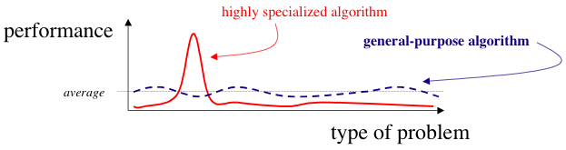
No Free Lunch Theorem

Wolpert and Macready (1997)

We have dubbed the associated results NFL theorems because they demonstrate that if an algorithm performs well on a certain class of problems then it necessarily pays for that with degraded performance on the set of all remaining problems.

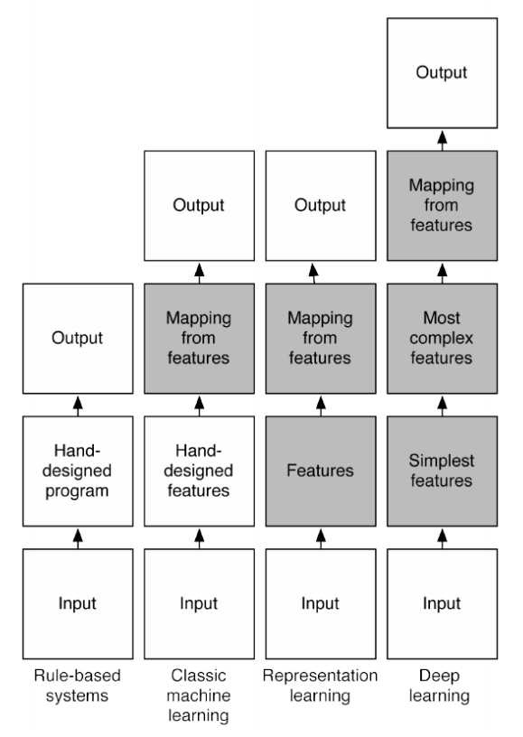
Classical ML v.s. Deep learning